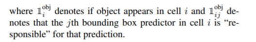
YOLO9000 bounding box를 예측하는데 dimension clusters anchor boxes로 사용한다.
4 coordinates for each bounding box
loss : sum of squared error loss
predicts an objectness score for each bounding box using logistic regression
threshold of .5
Faster RCCN과 달리 우리 시스템은 각 ground truth object 에 대해 하나의 bounding box를 할당한다.
2.2. Class Prediction
multilabel classification를 사용하여 bounding box에 포함될 수 있는 class를 예측한다.
softmax를 상요하지 않고 대신 단순한 independent logistic classifiers를 사용한다. softmax를 사용하면 각 bounding box가 겹치는 레이블이 많을 경우 잘 안된다.
학습하는 동안 class predictions 을 위해 binary cross entropy loss을 사용한다.
A multilabel approach better models the data. ⇒ 겹치는 label에 대하여
2.3. Predictions Across Scales
boxes는 3가지 다른 scale에 대해서 예측한다.
we predict 3 boxes at each scale so the tensor is N × N × [3 ∗ (4 + 1 + 80)] for the 4 bounding box offsets, 1 objectness prediction, and 80 class predictions.
다음으로 우리는 previous layer 2개에서 feature map을 가져와 2x upsample 한다. 또한 network의 초기에서 feature map을 가져와 연결을 사용하여 upsampled 된 feature와 concatenation한다. ⇒ 이 방법을 사용하여 upsampled feature에서 더 의미 있는 의미 정보를 얻고 이전 feature map에서 더 세분화된 정보를 얻을 수 있다.
Feature Pyramid Network
We then add a few more convolutional layers to process this combined feature map, and eventually predict a similar tensor, although now twice the size.
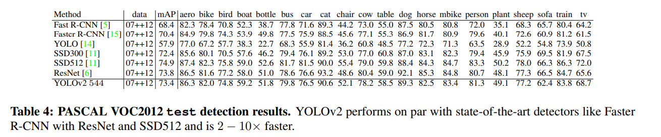
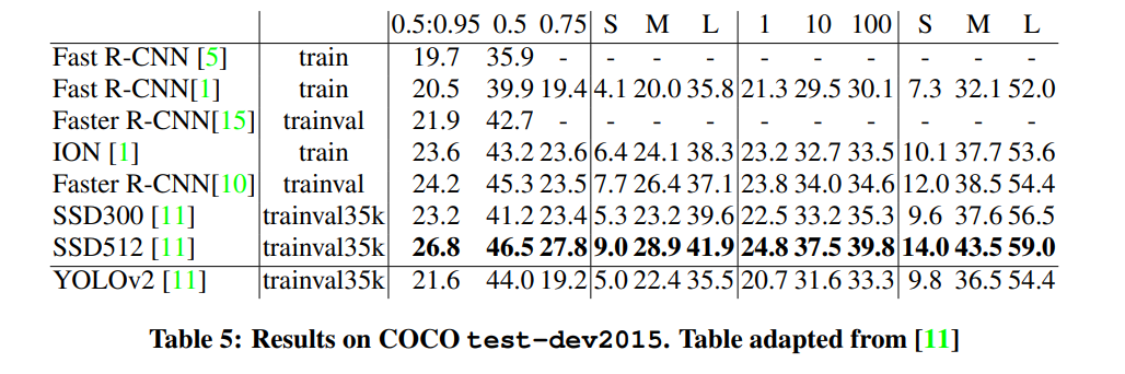
개선된 모델 YOLOv2는 PASCAL VOC and COCO 같은 standard detection tasks 에 대한 state-of-the-art 이다.
새롭고 다양한 규모의 학습 방법을 사용하면 동일한 Yolov2 모델을 다양한 sizes로 실행할 수 있으므로 속도와 정확도 사이에서 쉽게 trade-off 할 수 있따.
VOC 2007에서 67 FPS이고 76.8 mAP, 40 FPS에서 78.6 mAP를 획득하는 ResNet및 SSD를 사용하는 Faster RCNN과 함께 state-of-the-art methods 을 능가하는 동시에 훨씬 더 빠르다.
jointly train on object detection and classification ⇒ YOLO9000 을 COCO detection dataset과 ImageNet Classification dataset을 이용해 동시에 학습시킨다. 000개 이상의 서로 다른 개체 범주에 대한 탐지를 예측가능하며 여전히 실시간으로 실행된다.
1. Introduction
General purpose object detection 빠르고 정확하며 다양한 물체를 인식할 수 있어야 한다. fast and accurate을 증가 하였지만 여전히 a small set of objects제한이 있다.
현재의 object detection datasest는 classification 및 tagging 지정과 같은 other tasks을 위한 dataset에 비해 제한적이다.
hierarchical view of object classification
joint training algorithm, classification images to increase its vocabulary and robustness 활용하여 objects를 정확하게 지역한하는 방법을 학습
YOLO9000 a real-time object detector 9000 종에 대해서 할 수 있따.
YOLOv2, a state-of-the-art, real-time detector
our dataset combination method and joint training algorithm to train a model on more than 9000 classes from ImageNet as well as detection data from COCO
Fast R-CNN과 비교한 YOLO의 Error analysis 은 Yolo 가 상단한 localization error 를 발생시킨다.
YOLO has relatively low recall compared to region proposal-based methods
따라서 우리는 분류 정확도를 유지하면서 recall과 localization를 개선하는 데 주로 중점을 둡니다.
larger, deeper networks 경향이 있다. 더 좋은 성능은 더 큰 network를 훈련하거나 여러 model을 함께 앙상블 하는데 달려있다. 그러나 Yolov2를 사용하면 여전히 빠른 더 정확한 detector가 필요한다. network를 확장하는 대신 network를 단순화한 다음 representation을 더 쉽게 배울 수 있도록 한다.
다양한 아이디어를 사용
Batch Normalization
다른 형태의 regularization에 대한 필요성을 제거하면서 수렴을 크게 향상시킨다. 모든 convolution layer에 batch normalization을 추가하면 mAP를 2% 향상시켰다. 모델을 정규화 하는데도 도움이 되고 overfitting 없이 dropout 를 제거할 수 있따.
High Resolution Classifier
YOLO classifier network를 224x224에 학습한 다음 448x448 의 해상도에서 detection network를 학습하였다. object detection을 학습하면서 동시에 새로운 input resolution 에 적용해야 하는 것을 의미한다.
YOLOv2 classifier network ImageNet full 448 × 448 resolution 10 epoch → 이는 network 가 더 높은 resolution input에서 더 잘 작동하도록 filter를 조정할 시간을 준다. 그다음에 fine tune the resulting network on detection. mAP를 4% 향상시켰다.
Convolutional With Anchor Boxes
Yolo는 convolutional feature extractor 위에 fully -connected layer를 통해 직접 bounding box 좌료를 예측, 우리는 Yolo에서 fully-connected layer를 제거하고 bounding box 예측을 위해 anchor box를 사용한다. pooling layer를 제거하고 network의 convolution layer의 출력을 더 높은 해상도로 만든다. 448 x 448 대신 416개의 input image에서 작동하도록 network에서 축소한다.
a single center cell 을 갖는 feature map을 위해 홀 수 개의 위치를 갖는다 . 이는 큰 물체는 이미지의 중앙을 차지하는 경향이 있으므로 모두 근처에 있는 4개 위치 대신 이런한 물체를 예측하기 위해 중앙에 단일 위치를 갖는 것이 좋다. YOLO의 convolutional layer는 32배 만큼 이미지를 downsampling하므로 416 input image를 사용하여 13x13 출력 feature map을 얻는다. ⇒ 조금 더 작은 물체
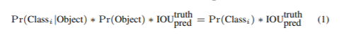
anchor box로 이동할 때 class prediction mechanism 을 spatial location 에서 분리하고 대신 모든 anchor box에 대한 class와 객체성을 예측한다. Yolo에 이어 objectness prediction 은 여전히 ground truth의 IOU를 예측하고 제안된 box 및 class predictions은 object가 있는 경우 해당 class의 conditional probablility 을 예측한다.
Anchor box를 사용하면 정확도가 약감 감소한다. Yolo는 이미지당 98(772)개의 box만 예측하지만 anchor box는 천 개 이상을 예측한다. anchor boxes가 없으면 중간 모델은 81%의 recall과 함께 69.5mAP를 얻는다. mAP가 감소하더라도 recall의 증가는 우리 모델이 개선할 여지가 더 많다는 것을 의미한다. ⇒ recall이 좋아졌다는 의미는 물체를 더 잘 찾아난다는 것이기 때문에 성능만 조금 더 개선하면 improve 한다는 여지가 있다.
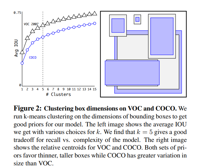
Dimension Clusters
box dimension는 수동적으로 결정하였따. ⇒ k-Means Clustering 방법으로 개선
Euclidean distance와 함께 standard k-means clustering을 사용하는 경우 큰 box는 작은 box보다 더 많은 오류를 생성한다. 그러나 원하는 것은 box의 크기와 무관한 좋은 IOU scores로 이어지는 사전 순위이다. distance metric
d(box,centroid)=1−IOU(box,centroid)
k= 5가 모델의 recall vs. model complexity 에 대해 좋은 tradeoff을 제공한다는 것을 발견하였다.
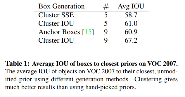
Cluster SSE (Sum of Square Error) 5
anchor box를 9개에서 5개로 줄임,
9개의 Cluster IOU를 사용하면 훨씬 더 높은 IOU를 볼 수 있다. 이것은 bounding box 를 생성하기 위해 k-평균을 사용하면 더 나은 representation으로 model을 시작하고 task을 더 쉽게 학습할 수 있다.
Cluster SSE (Sum of Square Error) 5
anchor box를 9개에서 5개로 줄임,
9개의 Cluster IOU를 사용하면 훨씬 더 높은 IOU를 볼 수 있다. 이것은 bounding box 를 생성하기 위해 k-평균을 사용하면 더 나은 representation으로 model을 시작하고 task을 더 쉽게 학습할 수 있다.
Direct location prediction
anchor box의 문제점 2: model instability 특히 초기 iteration 동안
원인은 : box의 (x,y)위치를 예측하는데서 발생 ,
region proposal networks에서 network는 tx및 ty값을 예측하고 (x,y) center coordinates는 다음과 같이 계산한다.
x=(tx∗wa)−xa
y=(ty∗ha)−ya
이 공식은 제한이 없으므로 bounding box를 예측한 위치에 관계 없이 모든 anchor box가 image의 어느 지점에서나 깥날 수 있다. random 초기화 를 사용하면 model이 합리적인 offset을 예측하기 위해 안정화되는데 오랜 시간이 걸린다.
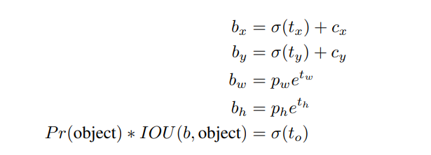
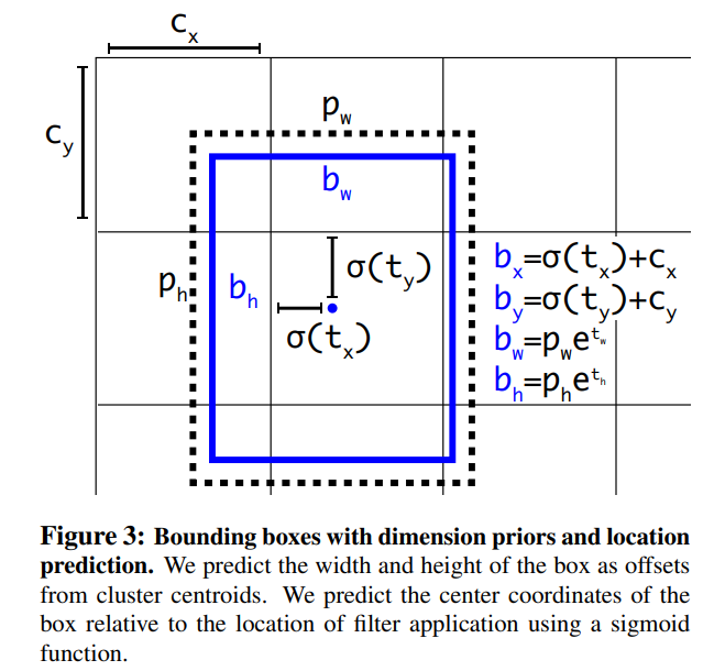
각 cell에 5개의 bounding box 예측
5 coordinates : tx, ty, tw, th, and to
cell의 image의 left corner (cx,cy)만큼 offset되고 bounding box 이전의 width와 height가 pw, ph 인 경우 예측은 다음과 같다.
pw,ph: anchor box의 너비 및 높이
bounding box center location을 directly predicting 하는 것과 함께 Dimension clustering을 사용하면 anchor box가 있는 버전보다 5%의 성능 향상된다.
Fine-Grained Features
passthrough layer
26 × 26 × 512 feature map → 13 × 13 × 2048 feature map → 큰물체 작은 물체를 더 잘 뽑아내게
13 × 13 × 2048 feature map 큰 물체를 탐지 못할 수 있다.
1% performance increase
YOLO v2의 13x13 feature map은 큰 물체를 탐지하는데 충분할 수 있으나 작은 물체를 잘 탐지하지 못 할 수 있다. 이를 해결하기 위해 13x13 feature map을 얻기 전의 앞 쪽의 layer에서 26x26 해상도의 feature map을 passthrough layer를 통해 얻는다.
사진 4. fine-grained features
위의 사진 4와 같이 26x26x512 -> 13x13x2048로 분해한 후 기존의 output인 13x13 feature map과 concatenate를 수행한다. 이러한 방법으로 1%의 성능을 향상시켰다.
Multi-scale Training
multi-scale training {320, 352, ..., 608}. 32배 사이즈로 다양하게 학습 ⇒ 같은 network인데 다양한 resolution을 예측할 수 있다.
Further Experiments.
3. Faster
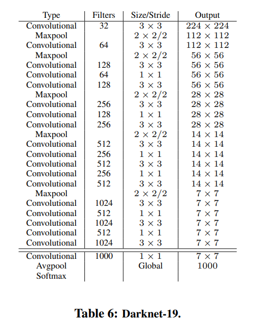
Darknet-19을 backbone network로 사용한다.
VGG-16 대신 Googlenet architecture을 사용 Googlenet architecture 속도가 더 빠르지만 정확도가 조금 낮다.
Darknet-19
VGG와 비슷(3 × 3 filters 사용)
Network in Network (NIN) 작업에 이어 global average pooling 을 사용하여 predictions를 수행하고 1 × 1 filters 를 사용하여 3 × 3 convolutions 사이의 특징 표현을 압축한다. 훈련을 안정화하고 수렴 속도를 높이며 모델을 정규화하기 위해 batch normalization를 사용한다.
19 convolutional layers and 5 maxpooling layers.
Training for classification
ImageNet 1000 class classification dataset 160 epochs
g stochastic gradient descent, learning rate 시작은 0.1,
polynomial rate decay with a power of 4
weight decay of 0.0005
momentum 0.9
standard data augmentation : random crops, rotations, and hue, saturation, and exposure shifts.
224x224 해상도로 학습한 후 448로
fine tuning : 위의 parameter 사용 , 10 epochs , learning rate of 10−3
Training for detection
last convolutional layer을 제거하고 3개의 3 × 3 convolutional layers with 1024 filters each followed by a final 1 × 1 convolutional layer with the number of outputs we need for detection.
4. Stronger
jointly training on classification and detection data.
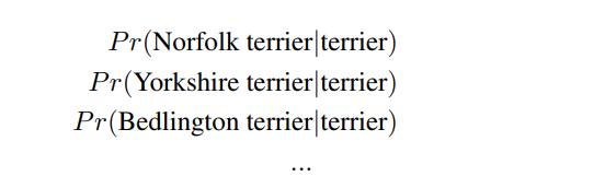
Hierarchical classification : 계층적인 분류를 사용한다.
WordNet는 data구조이고 tree는 아니다.
softmax
Hierarchical classification
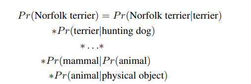
조건부 확률고 계산
absolute probability for 특정 node
P r(physical object) = 1.
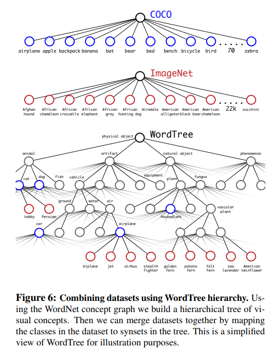
Dataset combination with WordTree
Joint classification and detection
Yolo9000
output size를 제한하기 위해 5개 대신 3개만 사용
detection backpropagate loss as normal
classification loss only classification loss is backpropagated at or above the corresponding level of the label.
5. Conclusion
real-time detection system YOLOv2 and YOLO9000
Yolov2 state-of-the-art faster , accuracy
YOLO9000 a real-time framework jointly optimizing detection and classification WordTree
우리는 물체 탐지에 대한 새로운 접근 방식인 YOLO를 제시한다. object detection 에 대한 사전 작업에서는 classifiers를 용도 변경하여 탐지를 수행하였다.
대신, 우리는 공간적으로 분리된 경계 상자 및 관련 클래스 확률에 대한 회귀 문제로 객체 탐지를 프레임화한다.
single neural network 은 하나의 평가에서 전체 이미지에서 직접 경계 상자와 클래스 확률을 예측한다.Since the 전부의 detection pipeline is a single network, it can be optimized end-to-end directly on detection performance.
우리의 통일된 architecture 매우 빠르다.
YOLO model 45 frames per second 로 이미지를 실시간으로 처리한다.
더 작은 네트워크 버전인 Fast YOLO, 놀랍게도 초당 155 frames per second 을 처리하고 다른 실시간 검출기의 두 배 이상의 mAP를 달성한다.
다른 sota detection 시스템과 비교할때 , YOLO는 오류를 더 많이 발생시키지만 그러나 백그라운드에서 잘못된 긍정을 예측할 가능성은 낮다.
마지막으로, YOLO는 객체의 매우 일반적인 표현을 학습한다.
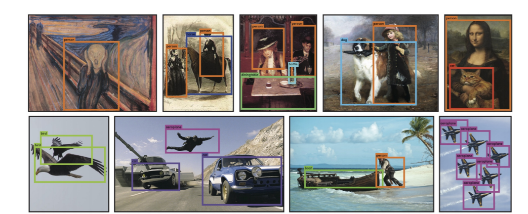
자연 이미지에서 예술작품과 같은 다른 도메인으로 일반화할 때 DPM 및 R-CNN을 포함한 다른 탐지 방법을 능가한다.
1. Introduction
인간은 이미지를 흘끗 보고, 이미지 안에 어떤 물체가 있는지, 어디에 있는지, 어떻게 상호작용하는지 즉시 알게 된다.
인간의 시각 시스템은 빠르고 정확하여 운전과 같은 복잡한 작업을 거의 의식하지 않고 수행할 수 있다.
물체 감지를 위한 빠르고 정확한 알고리즘을 통해 컴퓨터는 특수 센서 없이 자동차를 운전할 수 있고 보조 장치가 인간 사용자에게 실시간 장면 정보를 전달할 수 있으며 범용 반응형 로봇 시스템의 가능성을 열 수 있다.
현재 탐지 시스템은 분류기의 용도를 변경하여 탐지를 수행한다.
object를 탐지하기 위해 이러한 시스템은 해당 object에 대한 분류기를 가져와서 테스트 이미지의 다양한 위치와 척도에서 해당 object를 평가한다.
deformable parts models (DPM)과 같은 시스템에서는 분류기가 전체 이미지에 걸쳐 일정한 간격으로 실행되는 sliding window 접근 방식을 사용합니다.
R-CNN과 같은 보다 최근의 접근 방식은 region proposal methods 을 사용하여 먼저 이미지에서 potential bounding boxes 를 생성한 다음 이러한 제안된 상자에서 classifier를 실행한다. (2-stage)
분류 후 post-processing 는 bounding boxes 를 세분화하고 중복 탐지를 제거하며 장면의 다른 개체를 기반으로 상자를 다시 찾는 데 사용됩니다
이런 복잡한 pipeline은 각 개별 구성요소가 별도로 훈련되어야 하기 때문에 속도가 느리고 최적화하기 어렵다.
우리는 object detection 를 이미지 픽셀에서 경계 상자 좌표 및 클래스 확률에 이르기까지 단일 회귀 문제로재구성한다. 이 YOLO system을 사용하면 이미지를 한 번만(YOLO) 보고 어떤 개체가 있는지, 어디에 있는지 예측할 수 있다.
YOLO 는 매우 간단하다. Figure 1 참조
Figure 1: The YOLO Detection System. Processing images with YOLO is simple and straightforward. Our system (1) resizes the input image to 448 × 448, (2) runs a single convolutional network on the image, and (3) thresholds the resulting detections by the model’s confidence.
Figure 1: The YOLO Detection System. Processing images with YOLO is simple and straightforward. Our system
(1) resizes the input image to 448 × 448,
(2) runs a single convolutional network on the image
(3) thresholds the resulting detections by the model’s confidence.
A single convolutional network 는 해당 상자에 대한 여러 경계 상자와 클래스 확률을 동시에 예측한다. (1-stage)
YOLO는 전체 영상에 대해 훈련하고 탐지 성능을 직접 최적화한다.
이 통합 모델은 기존의 객체 감지 방법보다 몇 가지 이점이 있다.
첫째, YOLO는 매우 빠르다.
탐지를 회귀 문제로 간주하기 때문에 복잡한 파이프라인이 필요하지 않는다.
우리는 detection을 예측하는데 test 단계에서 새로운 이미지를 Yolo neural network에 넣어주기만 하면 간단하게 실행할 수 있다.
YOLO의 base network는 Titan X GPU에서 배치 처리 없이 초당 45프레임으로 실행되며 빠른 버전은 150fps 이상에서 처리한다.이 방식으로 우리는 video 를 실시간으로 할 수 있다는 것이다. 지연 시간이 25 milliseconds 미만이다. 또한 YOLO는 다른 실시간 시스템의 mAP의 2배 이상을 달성한다.
둘째, YOLO는 예측을 할 때 이미지에 대해 globally으로 추론한다. sliding window 및 d region proposal-based techniques과 달리, YOLO는 훈련 및 테스트 시간 동안 전체 이미지를 보기 때문에 클래스와 그 외관에 대한 상황 정보를 암시적으로 인코딩한다.
Fast R-CNN a top detection method 는 더 큰 컨텍스트를 볼 수 없기 때문에 이미지의 백그라운드 patches를 object로 착각한다.
YOLO는 Fast R-CNN에 비해 백그라운드 오류 횟수의 절반에도 미치지 못한다.
셋째, YOLO는 generalizable representations of objects을 학습한다. (일반화)
자연 이미지에 대해 훈련하고 예술작품에 대해 시험했을 때, YOLO는 DPM 및 R-CNN과 같은 상위 탐지 방법을 큰 폭으로 능가한다. YOLO는 매우 일반적이기 때문에 새로운 도메인이나 예기치 않은 입력에 적용될 때 분해될 가능성이 적다.
YOLO는 여전히 sota detection 시스템에 뒤처져 있다. 이미지의 object를 빠르게 식별할 수 있지만 일부 개체, 특히 작은 개체의 위치를 정확하게 지정하기 위해 고군분투하고 있다.
우리는 우리의 실험에서 이러한 트레이드오프를 더 자세히 조사한다.
우리의 모든 교육 및 테스트 코드는 오픈 소스이다. 다양한 사전 교육을 받은 모델도 다운로드할 수 있다.
2. Unified Detection
우리는 물체 탐지의 개별 구성 요소를 single neural network으로 통합한다. 우리 네트워크는 전체 이미지의 기능을 사용하여 각 경계 상자를 예측한다. 또한 모든 클래스의 모든 경계 상자를 동시에 예측한다. 이는 전체 이미지와 이미지의 모든 개체에 대한 네트워크 상의 이유를 의미한다. YOLO 설계는 높은 평균 정밀도를 유지하면서 종단 간 훈련end-to-end training 과 실시간 속도를 가능하게 한다.
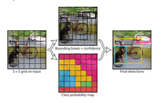
우리 시스템은 입력 이미지를 S × S grid로 나눈다. object 의 중심이 grid cell 로 떨어지면 해당 grid cell이 해당 object를 탐지한다.
각 grid cell 셀은 B 경계 상자와 해당 상자에 대한 신뢰 점수를예측한다.이러한 신뢰도 점수는 상자에 개체가 포함되어 있다는 모형의 신뢰도와 상자가 예측되는 정확도를 반영한다.
공식적으로 confidence 를 아래와 같이 정희 한다.
해당 cell 에 object 가 없으면 confidence는 0이다.
그렇지 않으면 신뢰 점수가 예측 상자와 실제 실측 사이의 intersection over union (IOU) 과 같기를 원한다.
각 경계 상자는 x, y, w, h, 5개의 예측으로 구성된다. (x, y) 좌표는 그리드 셀의 경계를 기준으로 상자의 중심을 나타낸다.
width and height 는 전체 이미지에 대해 예측된다. 마지막으로 신뢰 예측은 예측 상자와 모든 실제 실측 상자 사이의 IOU를 나타낸다.
Each grid cell also predicts C conditional class probabilities
이러한 확률은 개체를 포함하는 gird cell에서 조건화된다. 우리는 상자 B의 수에 관계없이 gird cell당 하나의 클래스 확률 집합만 예측한다.
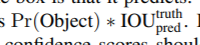
test time 에서 우리는 the conditional class probabilities and the individual box confidence predictions 를 곱한다.
각 상자에 대한 class-specific confidence scores를 제공한다. 이러한 점수는 상자에 해당 클래스가 나타날 확률과 예측 상자가 개체에 얼마나 적합한지 인코딩한다.
Figure 2: The Model. Our system models detection as a regression problem. It divides the image into an S × S grid and for each grid cell predicts B bounding boxes, confidence for those boxes, and C class probabilities. These predictions are encoded as an S × S × (B ∗ 5 + C) tensor.
For evaluating YOLO on PASCAL VOC, we use S = 7, B = 2. PASCAL VOC has 20 labelled classes so C = 20. Our final prediction is a 7 × 7 × 30 tensor.
2.1. Network Design
a convolutional neural network
evevaluate datasetsdetection dataset : PASCAL VOC
fully connected layers 이 output probabilities and coordinates 를 예측하는 동안 network extract features의 initial convolutional layers은 이미지에서 특징을 나타낸다.
우리의 네트워크 아키텍처는 이미지 분류를 위한 GoogleLeNet 모델에서 영감을 받았다.
Our network has 24 convolutional layers followed by 2 fully connected layers.
Instead of the inception modules used by GoogLeNet, we simply use 1 × 1 reduction layers followed by 3 × 3 convolutional layers
The full network is shown in Figure 3.
Figure 3: The Architecture. Our detection network has 24 convolutional layers followed by 2 fully connected layers. Alternating 1 × 1 convolutional layers reduce the features space from preceding layers. We pretrain the convolutional layers on the ImageNet classification task at half the resolution (224 × 224 input image) and then double the resolution for detection.
우리는 또한 fast object detection의 boundaries 를 밀어 넣도록 설계된 빠른 버전의 YOLO를 훈련시킨다.Fast YOLO는 더 적은 컨볼루션 레이어(24개 대신 9개)와 더 적은 필터를 가진 신경망을 사용한다.네트워크의 크기를 제외한 모든 교육 및 테스트 파라미터는 YOLO와 Fast YOLO 간에 동일하다.
network의 최종 output 은 7 × 7 × 30 tensor of predictions.
2.2. Training
우리는 ImageNet 1000 클래스 경쟁 데이터 세트에서 컨볼루션 레이어를 pretrain하였다.
pretraining 을 위해 we use the first 20 convolutional layers from Figure 3 followed by a average-pooling layer and a fully connected layer. 우리는 이 네트워크를 약 일주일 동안 훈련시키고, Cafe's Model Zoo [24]의 GoogleLeNet 모델과 비교할 수 있는 ImageNet 2012 검증 세트에서 88%의 단일 크롭 top-5 정확도를 달성한다 .
우리는 모든 훈련과 추론에 Darknet framework를 사용한다.
그런 다음 모델을 변환하여 탐지를 수행한다. Ren et al. pretrained networks 에 컨볼루션 계층과 연결된 계층을 모두 추가하는 것이 성능을 향상시킬 수 있음을 보여준다. 이들의 예에 따라, 우리는 무작위로 초기화된 가중치를 가진 four convolutional layers and two fully connected layers 를 추가한다. 탐지에는 종종 세분화된 시각적 정보가 필요하므로 네트워크의 입력 해상도를 224 × 224에서 448 × 448로 증가시킨다.
우리의 최종 레이어는 class probabilities and bounding box coordinates 모두 예측한다. We normalize the bounding box width and height by the image width and height so that they fall between 0 and 1. 0 ~ 1 사이로 normalze한다.We parametrize the bounding box x and y coordinates to be offsets of a particular grid cell location so they are also bounded between 0 and 1. 0 ~ 1 사이로 다 한다. w,h , x,y
우리는 최종 계층에 linear activation function를 사용하고 다른 모든 계층은 다음과 같은 leaky rectified linear activation 를 사용한다.
우리는 모델의 출력에서 sum-squared error 를 최적화한다. 우리는 최적화하기 쉽기 때문에 sum-squared error 를 사용하지만 maximizing average precision 한다는 우리의 목표와 완벽하게 일치하지는 않는다. 이것은 localization error를 이상적이지 않을 수 있는 분류 오류와 동등하게 weights를 부여한다.또한 모든 이미지에서 많은 grid cells에는 object가 없다. 이것은 그 cells들의 "confidence" 점수를 0으로 밀어넣고, 종종 물체를 포함하고 있는 cells로부터의 gradient를 압도한다. 이는 모델 불안정성을 초래하여 훈련 초기에 분산될 수 있다.
이를 해결하기 위해 경계 상자 좌표 예측에서 손실을 늘리고 개체를 포함하지 않는 상자에 대한 신뢰 예측에서 손실을 줄인다.
있는것은 5 없는 것은 0.5로 한다.
또한 Sum-squared error 는 large boxes and small boxes의 오차의 가중치를 동일하게 부여한다. 우리의 error metric 은 큰 상자의 작은 편차가 작은 상자보다 덜 중요하다는 것을 반영해야 한다.이를 부분적으로 해결하기 위해 우리는 폭과 높이가 아니라 경계 상자 폭과 높이의 제곱근을 예측한다.
YOLO predicts multiple bounding boxes per grid cell. 여러개의 bouding boxes를 예측한다. 학습 시에는 경계 상자 예측 변수 하나가 각 개체에 대해 책임을 지기를 원한다. 우리는 예측이 실제와 함께 가장 높은 전류 IOU를 갖는 물체를 예측하는 데 "responsible"을 가진 one predictor 을 할당한 between the bounding box predictor에 specialization 로이끈다. Each predictor gets better at predicting certain sizes, aspect ratios, or classes of object, improving overall recall. =>ertain sizes, aspect ratios, or classes of object
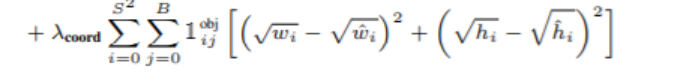
training 중에, 다음과 같은 multi part loss function 를 최적화한다.
Note that the loss function only penalizes classification error if an object is present in that grid cell (hence the conditional class probability discussed earlier). => classification error은 grid cell에 object 있을 경우
It also only penalizes bounding box coordinate error if that predictor is “responsible” for the ground truth box (i.e. has the highest IOU of any predictor in that grid cell). => box predictor 가 ground truth box “responsible” 인경우에만 bounding box coordinate error penalizes
yolov1 loss :
여기서 root를 하는 경우는 작은 물체와 큰 물체가 차이 나기 때문이다.
큰 강아지와 작은 강아지의 loss 차이가 같은 경우에 큰 강아지는 조금만 차이 나는데 작은 강아지 일 경우에는 머리 부분 거의 차이이다. 하지만 loss차이는 같다. => 해결은 root를 해준다. => 작은 object에 대해서 큰 loss를 해준다.
0.5로 곱하는 이유는 :
S = 7 이고 b가 2일 경우에 실제 예측은 7*7*2 = 98개 predict를 한다.
object가 없는 경우가 더 많고 object가 많을 경우 gradient 에 영향을 주어서 0.5를 곱해서 수치를 좀 낮추어서 object 있는 것과 없는 것의 차이를 줄인다.
5를 곱하는 이유는 :
위치를 더 정확하게 할려고 5를 곱한다.
135 epochs
training and validation data sets from PASCAL VOC 2007 and 2012
When testing on 2012 we also include the VOC 2007 test data for training.
batch size 64
momentum 0.9
decay 0.0005
learning rate 은 epoche에 달라 다르게 했다.
높은 학습 속도로 시작하면 불안정한 gradient로 인해 모델이 종종 분리된다.
overfitting을 피하기 위해 dropout and extensive data augmentation
A dropout layer with rate = .5 after the first connected layer prevents co-adaptation between layers.
co-adaptation: 상호적응 문제는,신경망의 학습 중,어느 시점에서 같은 층의 두 개 이상의 노드의 입력 및 출력 연결강도가 같아지면,아무리 학습이 진행되어도 그 노드들은 같은 일을 수행하게 되어 불필요한 중복이 생기는 문제를 말한다.즉 연결강도들이 학습을 통해 업데이트 되더라도 이들은 계속해서 서로 같은 입출력 연결 강도들을 유지하게 되고 이는 결국 하나의 노드로 작동하는 것으로써,이후 어떠한 학습을 통해서도 이들은 다른 값으로 나눠질 수 없고 상호 적응하는 노드들에는 낭비가 발생하는 것이다.결국 이것은 컴퓨팅 파워와 메모리의 낭비로 이어진다.
For data augmentation we introduce random scaling and translations of up to 20% of the original image size
또한 HSV 색 공간에서 이미지의 노출과 포도를 최대 1.5배까지 임의로 조정했다.
색상(Hue), 채도(Saturation), 명도(Value)
2.3. Inference
훈련과 마찬가지로 테스트 이미지에 대한 탐지를 예측하려면 네트워크 평가가 하나만 필요한다.
On PASCAL VOC the network predicts 98 bounding boxes per image and class probabilities for each box. => 98개 bounding box: 7(S) * 7 * 2( B). YOLO는 classifier-based methods과 달리 단일 네트워크 평가만 필요하기 때문에 테스트 시간에 매우 빠르다.
그리드 설계는 경계 상자 예측에서 공간 다양성을 시행한다.object 가 속한 grid cell이 명확하면 네트워크는 각 Object에 대해 하나의 상자만 예측한다. 하지만 , some large objects or objects near the border of multiple cells can be well localized by multiple cells. =>multiple cells 생길 수 있다.=> Non-maximal suppression로 해결할 수 있다. R-CNN 또는 DPM의 경우처럼 성능에 중요하지 않지만, 최대가 아닌 억제 기능은 mAP에서 23%를 추가한다.
2.4. Limitations of YOLO
각 grid cell 은 두 개의 상자만 예측하고 하나의 클래스만 가질 수 있기 때문에 YOLO는 bounding box predictions에 strong spatial constraints을 가한다. 이 spatial constraint은 우리 모델이 예측할 수 있는 가까운 객체의 수를 제한한다. Our model struggles with small objects that appear in groups, such as flocks of birds.=> 작은 물체에 대해서 성능을 올리려고 노력하고 있다.
우리의 모델은 데이터에서 경계 상자를 예측하는 방법을 배우기 때문에, 새로운 또는 특이한 가로 세로 비율이나 구성의 object 로 일반화하기가 어렵다. =>new or unusual aspect ratios or configurations 우리의 모델은 또한 우리의 아키텍처가 입력 이미지에서 여러 down-sampling layer을 가지고 있기 때문에 경계 상자를 예측하는 데 비교적 coarse features 을 사용한다.
마지막으로, detection performance 에 근사한 loss function 에 대해 훈련하는 동안, 우리의 loss function 는 작은 bounding boxes versuslarge bounding boxes 에서 오류를 동일하게 취급한다.큰 상자의 작은 오류는 일반적으로 양호하지만 작은 상자의 작은 오류는 IOU에 훨씬 더 큰 영향을 미친다. Our main source of error is incorrect localization.
3. Comparison to Other Detection Systems
Object detection is a core problem in computer vision. => 핵심문제이다.
Detection pipelines 은 일반적으로 입력 이미지에서 일련의 robust features 하는 것으로 시작한다.
Then, classifiers [36, 21, 13, 10] or localizers [1, 32] are used to identify objects in the feature space.
These classifiers or localizers are run either in sliding window fashion over the whole image or on some subset of regions in the image [35, 15, 39].
We compare the YOLO detection system to several top detection frameworks, 주요 유사점과 차이점을 강조한다.
Deformable parts models. sliding window DPM은 disjoint pipeline을 사용하여 static features을 추출하고 영역을 분류하며 점수가 높은 영역에 대한 경계 상자를 예측한다.우리의 시스템은 본질적으로 다른인 모든 부분을 단일 컨볼루션 신경망으로 교체한다. The network performs feature extraction, bounding box prediction, nonmaximal suppression, and contextual reasoning all concurrently. 네트워크는 static features in-line 기능을 학습하고 탐지 작업에 최적화한다. DPM보다 빠르고 더 정확하다.
R-CNN. R-CNN and its variants은 이미지에서 물체를 찾기 위해 sliding windows 대신 region proposals을 사용한다. Selective Search generates potential bounding boxes, a convolutional network extracts features, an SVM scores the boxes, a linear model adjusts the bounding boxes, and non-max suppression eliminates duplicate detections.이 complex pipeline의 각 단계는 독립적으로 정밀하게 조정되어야 하며 결과 시스템은 매우 느려서 테스트 시간에 영상당 40초 이상 걸린다.
YOLO는 R-CNN과 몇 가지 유사점을 공유한다.각 grid cell은 potential bounding boxes를 제안하고 convolutional features 을 사용하여 해당 상자에 점수를 매긴다. 그러나, 우리의 시스템은 동일한 객체에 대한 여러 탐지를 완화하는 데 도움이 되는 그리드 셀 제안에 spatial constraints을 가한다. 또한 우리 시스템은 선별 검색의 약 2000개보다 이미지당 98개만 훨씬 적은 경계 상자를 제안한다. 마지막으로, 우리의 시스템은 이러한 개별 구성요소를 공동으로 최적화된 단일 모델로 결합한다.
Other Fast Detectors
Deep MultiBox.
OverFeat.
MultiGrasp.
4. Experiments
먼저 YOLO를 PASCAL VOC 2007로 다른 실시간 detection 시스템과 비교한다.
YOLO와 R-CNN variants 의 차이를 이해하기 위해 우리는 YOLO가 만든 VOC 2007과 R-CNN의 최고 성능 버전 중 하나인 Fast R-CNN의 오류를 탐구한다. the different error profiles 을 기반으로 우리는 YOLO를 사용하여 Fast R-CNN 탐지를 다시 검색하고 백그라운드 잘못된 긍정에서 오류를 줄일 수 있다는 것을 보여줌으로써 상당한 효과를 얻을 수 있다.
또한 VOC 2012 결과를 제시하고 mAP를 현재의 sota 방법과 비교한다. 마지막으로 YOLO는 artwork dataset에 대해서도 other detectors 보다 더 좋은 결과로 일반화됨을 보인다.
4.1. Comparison to Other RealTime Systems
Fast YOLO is the fastest object detection method on PASCAL;
Fast R-CNN은 R-CNN의 classification 단계를 빠르게 했지만 selective search
mAP는 높지만 0.5 fps 로 실시간은 아니다.
최근의 Faster R-CNN은 bbox 를 제안하기 위해 selective search 대신 Szegedy 처럼 신경망을 사용한다.
테스트해본 결과 가장 정확한 모델이 7 fps 를 달성하고 덜 정확한 모델은 18 fps 이다. Faster
R-CNN의 VGG16 모델은 mAP 가 10이 더 높은데 YOLO보다 6배 느리다.
Faster R-CNN의 ZeilerFergus 모델은 YOLO보다 2.5 배만 느리지만 덜 정확하다.
4.2. VOC 2007 Error Analysis
YOLO와 다른 sota detector와 차이를 더 상세하게 조사하기 위해 VOC 2007 결과를 상세히 분석해본다.Fast R-CNN은 PASCAL에서 가장 성능이 뛰어난 검출기 중 하나이며 탐지를 공개적으로 사용할 수 있기 때문에 우리는 YOLO를 Fast RCNN과 비교한다.
우리는 Hoiem 등의 방법론과 도구를 사용한다.테스트 시 각 범주에 대해 해당 범주의 상위 N개 예측을 살펴분다. 각 예측은 정확하거나 오차 유형을 기준으로 분류된다.
• Correct: correct class and IOU > .5
• Localization: correct class, .1 < IOU < .5
• Similar: class is similar, IOU > .1
• Other: class is wrong, IOU > .1
• Background: IOU < .1 for any object
Figure 4: Error Analysis: Fast R-CNN vs. YOLO These charts show the percentage of localization and background errors in the top N detections for various categories (N = # objects in that category).
4.3. Combining Fast R-CNN and YOLO
Table 2: Model combination experiments on VOC 2007. We examine the effect of combining various models with the best version of Fast R-CNN. Other versions of Fast R-CNN provide only a small benefit while YOLO provides a significant performance boost.
4.4. VOC 2012 Results
Table 3: PASCAL VOC 2012 Leaderboard. YOLO compared with the full comp4 (outside data allowed) public leaderboard as of November 6th, 2015. Mean average precision and per-class average precision are shown for a variety of detection methods. YOLO is the only real-time detector. Fast R-CNN + YOLO is the forth highest scoring method, with a 2.3% boost over Fast R-CNN.
4.5. Generalizability: Person Detection in Artwork
Figure 5: Generalization results on Picasso and People-Art datasets.
Figure 6: Qualitative Results. YOLO running on sample artwork and natural images from the internet. It is mostly accurate although it does think one person is an airplane.
6. Conclusion
YOLO라는 통합 모델을 도입했는데 구축이 단순하고 학습은 전체 이미지에서 직접 이루어진다. classifier 기반의 방법과 달리 YOLO는 detection 성능에 직접 연관된 손실함수로 학습되고 전체 모델은 결합되어 학습된다.
Fast YOLO는 말그대로 가장 빠른 일반 목적의 사물 detection 시스템이며 YOLO는 최고의 실시간 detection 으로 등극했다. YOLO는 또한 빠르고 강건한 detection 에 의존하는 각종 응용들을 이상적으로 만드는 새로운 영역으로까지 일반화되고 있다.