CDistNet: Perceiving Multi-Domain Character Distance for Robust Text Recognition

https://arxiv.org/abs/2111.11011

Abstract

attention-based encoder-decoder framework는 scene text recognition에서 인기가 있는 이유는 visual and semantic domains으로 부터 recognition clues(힌트)를 통합하는데 있어서 성능이 우월하다. ⇒ scene text recognition 의 trend이다.

하지만 최근의 연구는 visual and semantic 양쪽의 clues가 특히 어려운 text에서 서로 잘 연결이 안되고 그것을 완화하기 위해서 character position constraints 을 소개한다. ⇒ 한계점

어떤한 성공에도 불구하고 의미 있는 지역적인 image regions와 a content-free positional embedding은 거의 안정적으로 연결되지 않는다.

이 논문은 visual and semantic related position encoding 새로운 모듈을 소개 ⇒ Multi-Domain Character Distance Perception (MDCDP)이라고 하는 모듈

MDCDP는 attention mechanism에 따라 visual and semantic features 두개 다 query로 사용하기 위해 positional embedding을 사용한다.

visual and semantic distances 를 모두 설명하는 positional clue를 자연스럽게 encoding한다.

우리는 새로운 architecture CDistNet이라고 하고 MDCDP를 여러개 쌓은 것 이며 좀 더 정확한 distance modeling이 가능하다.

따라서 다양한 어려움이 제시되더라도 visual-semantic alignment 이 잘 구축된다.

two augmented datasets and six public benchmarks

시각화는 또한 CDistNet이 visual and semantic domains 모두 에서 적절한 attention localization를 달성함을 보여준다.

소스코드 위치 : https://github.com/ simplify23/CDistNet. 소스코드는 초반에 없었는데 공개되였다.

1. Introduction

최근 몇년 동안 엄청나는 많은 연구가 수행되었음에도 Scene text recognition은 여러가지 문제에 직면해있다. 예를 들어, complex text deformations, unequally distributed characters, cluttered background, etc. ⇒ key issue

최근에는 attention-based encoder-decoder methods가 이 task에서 인상적인 영향을 보여왔다.

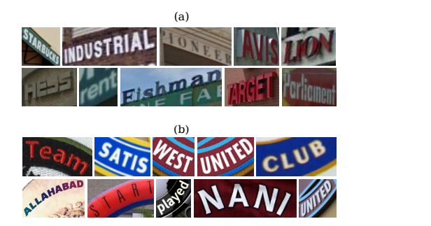
하지만 최근 연구[38]에서 는 두가지 잘못 인식된 예와 같이 흔치 않는 정형화 되지 않는 text에서 mismatch가 쉽게 일어난다. Fig.1 (a)참조 .

선행 연구에서 mismatch 발생한 원인

1). visual clue가 약할 때 visual counterpart에 대해서 semantic clue가 제대로 찾지 못한다.

2). 길이가 long text에서 많이 일어난다. text 길이가 길면 semantic feature가 점점 강화되면서 완전히 압도가 된다.

⇒ attention drift

위의 문제로 , mismatch를 완화하기 위하여 character position을 사용하여 연구를 진행한다 . sinusoidal-like positional embedding [6,29] or others [35,43,44]으로 encoding하였다.

이런 전략으로 문제는 좀 해결할 수 있으지만 [29, 44]여기에서는 content-free positional embedding을 사용하였기 때문에 visual feature가 character position하고 안정적으로 연관짓기가 어려웠다. 게다가 이미지 위치에 대한 character position에 대한 위치도 정해놓지 못하고 content-free positional embedding이 오히려 position order에 대한 제약만 주었다.

content-aware receptor를 해서 인식하는 것이 아니라 position order에 대한 제안만 주었다.

게다가 position and semantic space 관계는 아예 무시를 해버린다.

이 논문에서는 앞에서 언급된 이슈들을 극복하기 위해서 Multi Domain Character Distance Perception (MDCDP) 이라고 하는 새로운 module을 개발하였다.

기존의 연구 [34, 44] 와 유사하게 fixed positional embedding이 초기화 된다.

하지만 다른 점은 encoder가 position embedding하고 나서 그리고 visual and semantic features가 self-attention enhancement를 걸친다. 그리고 나서 비로서 query vector로 사용이 된다.

two enhanced features가 일종의 visual and semantic distance-aware representation 이 된다.

이전 정보 가 다음 MDCDP의 query vector로 들어간다. 그렇게 하면 좀 더 attention-focused visual-semantic alignment 가 얻어진다.

이런 idea를 따라서 CDistNet이라는 architecture를 제안한다.

여러개 MDCDP가 쌓인 것이고 정확한 distance modeling이 가능하도록 한다.

이렇게 하면 complex character이 spatial layouts 이 인식하는데 도움이 된다.

(b) HA-IC13 and CA-IC13 datasets are created by horizontal and curved stretching ICDAR2013 with various scales.

(c) We develop CDistNet that perceives multi-domain character distance better by position-related joint encoding. Compared with baseline, the accuracy margin becomes larger as the deformation severity rises.

3가지 기여도가 이다.

1. MDCDP visual and semantic features모두 positional feature 를 사용 할 수 있게 만든다.
2. CDistNet stacks several MDCDP 어려운 text를 recognizing하는데 이점이 있다.
3. we carry out extensive experiments with different configurations and compare CDistNet with existing methods.

2. Related Work

2.1. Semantic-free Methods

RNN and CTC loss

semantic정보를 무시 하고

visual feature만 가지고 modeling한다.

2.2. Semantic-Enhanced Methods

visual feature을 강화하기 위해 semantic clue를 활용하고 attention framework와 함께 encoder decoder를 사용하는 것을 강조

Transformer [34], a powerful model in capturing global spatial dependence, many variants [23, 29, 37] were developed with improved accuracy.

semantic loss를 도입한 것도 있고

semantic feature를 사용하는데 visual feature를 강화하는

ABINet은 별도의 language model을 사용하고 나중에 합쳐서 사용

하지만 misalignment문제가 여전히 남아 있고 attention drift

2.3. Position-Enhanced Methods

position도 고려하겠다.

character position encoding to ease the recognition

advanced rectification models 개발하였지만 , rectification 자체로는 서로 different clues에서 synergistic사용하는데 실패하였다.

Transformer-based models attention mechanism was non-local global하게 한다.

sinusoidal positional embedding

learnable embedding

segmentation map : ensure that characters

RobustScanner [44] proposed a position enhancement branch along with a dynamical fusion mechanism and achieved impressive results.

RobustScanner content-free positional embedding that hardly built a stable correspondence between positions and local image regions

CDistNet에서는 positional embedding을 visual and semantic features 양족에다 주입해서 multi-domain distance aware modeling 수립

3. Methodology

end-to-end trainable network

attention-based encoder-decoder framework

encoder : three branches : encoding visual, positional and semantic information

decoder : three kinds of information are fused by a dedicated designed MDCDP module, positional branch is leveraged to reinforce both visual and semantic branches and generate a new hybrid distance-aware positional embedding.

The generated embedding, which records the relationship among characters in both visual and semantic domains, is used as the positional embedding of the next MDCDP. (다음 MDCDP input으로 사용)

It is thus conducive to generating a attention-focused visual-semantic alignment.

The MDCDP module is stacked several times in CDistNet to achieve a more precise distance modeling.

At last, characters are decoded sequentially based on the output of the last MDCDP module.

마지막 MDCDP module의 output이 문자를 순차적으로 decoding된다.

3.1. Encoder

Visual Branch. TPS를 사용해서 rectify 을 먼저 한다.

Backbone : ResNet-45 and Transformer units , both local and global spatial dependencies를 captures 한다.

ResNet45

Transformer units are three-layer self-attention encoders with 1024 hidden units per layer

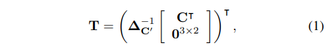
T : TPS block

R represents ResNet-45, ResNet-45 downsamples both the width and height to 1/8 of the original size

τ is the Transformer unit

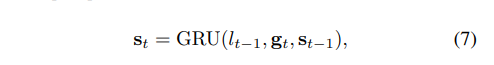
Semantic Branch.

previously seen characters during training

이전에 decode된 character들이 input으로 들어간다.

test 단계에서, 이전에 decode된 character들은 각 time step에서 update되는 current semantic feature으로 encode된다.

Embedding of the start token is used when decoding the first character.

L을 decoding할려고 하면 input은 없으면 안되서 start token으로 한다.

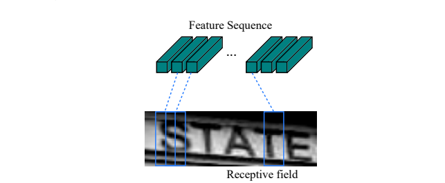
Positional Branch.

text의 문자 위치를 endode한다.

먼저 one-hot vector로 만든다. → same sinusoidal positional embedding

3.2. MDCDP

MDCDP module is formulated on the decoder side and benefit the recognition

3가지 parts로 구성이 되여있다.

self-attention enhancement for positional feature reinforcement

cross-branch interaction that utilizes positional feature to query both the visual and semantic branches, obtaining positional-enhanced representations

dynamic shared fusion to get a visual and semantic joint embedding

Self-Attention Enhancement (SAE)

encoder에서 positional embedding을 주면 SAE 가지고 embedding을 강화한다. multi-head self-attention block한개인 vanilla Transformer에서 다 빼고 하나인 것을 하고 self-attention을 한다.

dimension도 줄였다.

이 방식은 upper triangular mask 이고 

반대로 된 것은 lower triangular mask이다.

np.triu() ⇒ upper triangular mask : mask is applied to the query vector of the self-attention block to prevent from ”seeing itself”, or saying, leaking information across time steps. 다음 정보는 보면 안된다.

np.tril() ⇒ lowertriangular mask

RobustScanner내용

before using the positional embedding to query the visual feature 이러한 enhancement 는 사용하지 않는다. The query vector is always fixed in different character sequences. 바뀐 것이 없다.

반면에 , our enhancement enables a more targeted positional embedding learning.

Cross-Branch Interaction (CBI)

positional embedding is treated as the query vector

visual and semantic branches in parallel

When applying to the visual branch, it uses previous decoded character locations to search the position of the next character in the text image. CBI-V

While applying to the semantic branch, it models the semantic affinities between previous decoded characters and current positional clue. CBI-S.

Both branches have been reinforced after the interactions.

A similar upper triangular mask is also applied to the semantic branch to prevent information leaks due to its dynamical update nature.

이전 연구에서는 semantic feature가 query 로 들어가고

RobustScanner position에서 추가적인 query를 visual 쪽에 다 query를 얻은 것이다. position to visual and enables a positional-enhanced decoding.

하지만 , 우리는 semantic branch는 그대로 둔다. 대조적으로, we formulate the interactions as the positional-based intermediate enhancement to both visual and semantic domains. It reinforces not only visual but also semantic features and can be understood as delineating the multi-domain character distance.

Dynamic Shared Fusion (DSF).

two positional-enhanced features as input

visual 과 semantic

channel방향으로 concatenated 해서 하는데 channel이 2배가 된 hybrid feature가 된다.

→ 그 다음 다시 1 × 1 convolution 을 해서 절반으로 줄인다.

→ 그 다음 gating mechanism을 사용 transformed weight matrices

→ both visual and semantic features element-wisely

→ dynamic fusion

ABINet 

channel이 2C였다가 C로 줄어든다.

특이한 점은 the weights are shared among different MDCDP modules. As a consequence, DSF not only decouples the feature fusion with the previous attention learning, but also eases the network modeling.

4. Experiments

4.1. Datasets

three kinds of datasets :

two synthetic datasets for model training MJSynth (MJ) [10] and SynthText (ST) [7]

데이터 셋 sample

https://arxiv.org/pdf/1904.01906.pdf

two augmented datasets for model verification

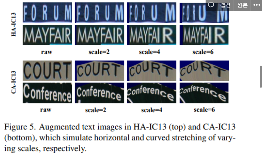
HA-IC13 and CA-IC13 two augmented datasets created from ICDAR2013

simulate the horizontal (HAIC13) and curved (CA-IC13) stretching with scales from 1 (the smallest deformation) to 6 (the largest deformation) with interval of 1 using the data augmentation tool in [21]

postprocessing exception 것을 처리 하기 위한 것

6배 정도 많다.

six widely used public datasets for both ablation study and comparison with existing methods.

ICDAR2013 (IC13) [13], Street View Text (SVT) [36], IIIT5k-Words (IIIT5k) [24], ICDAR2015 (IC15) [12], SVT-Perspective (SVTP) [26] and CUTE80 (CUTE) [28]

The first three mainly contain regular text while the rest three are irregular.

4.2. Implementation details

We resize the input images to 32×128 and employ data augmentation such as image quality deterioration, color jitter and geometry transformation.

 Transformer 확인 

transformer의 learning rate와 같다.

To reduce the computational cost, we shrink the transformer units employed, where dimension of the MLP layer is reduced from 2048 to 1024 in encoder, and from 2048 to 512 in decoder.

beam search

4.3. Ablation study

The number of MDCDP modules considered.

layer를 많이 쌓으면 쌓을 수록 computational cost가 증가한다.

Therefore the MDCDP modules in CDistNet are empirically set to 3.

The effectiveness of SAE.

self attention enhancement는 position branch 에 사용

The effectiveness of CBI.

The result basically validates two hypotheses.

First, imposing the positional clue is helpful.

Second, it is effective to query the semantic feature by using the positional clue, which perceives the semantic affinities between previous decoded characters and current position.

The effectiveness of DSF.

DSF outperforms static-based fusions (Add and Dot) as well as the scheme that not sharing weights among MDCDP modules.

4.4. Model Verification

Contribution of the positional utilization.

We first explain how the methods are modified.

CDistNet w/o Sem

Transformer* visual branch를 강화

RobustScanner* Transformer unit to replace the raw ”CNN+LSTM” implementation

CDistNet

With the modifications above, accuracy

gains from the position modeling can be quantitatively evaluated.

positional utilization이 중요

Performance on augmented datasets.

HAIC13 and CA-IC13 are simulated with different levels of horizontal and curved deformations.

It clearly verifies the advantage of CDistNet in recognizing difficult text.

Decoding Visualization.

attention map based on the positional-enhanced visual branch and give some examples in Fig.6

It again indicates the superiority of the proposed MDCDP module.

semantic affinities between previous decoded characters and current position in Fig.7

Analysis of good and bad cases.

good: we can conclude that CDistNet retains powerful and universal recognition capability with the existence of various difficulties, e.g., diverse text shapes, blur, distortions, etc.

bad : We also list some bad cases in Fig.9. The failures can be summarized as three categories mainly, multiple text fonts (cocacola, quilts), severe blur (coffee) and vertical text (garage). Most of them are even undistinguishable by humans and they are common challenges for modern text recognizers.

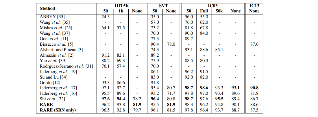
4.5. Comparisons with Existing Methods

five datasets including IC13, SVT, IIIT5K, IC15 and SVT-P when trained based on the two synthetic datasets.

irregular text datasets

5. Conclusion

extreme irregular text, we have presented the MDCDP module which utilizes positional feature to query both visual and semantic features within the attention-based encoder-decoder framework.

both visual and semantic domains.

MDCDP module

eight datasets that successfully validate our proposal.

The result on augmented datasets shows larger accuracy margin is observed as the severity of deformation increases.

ablation studies

state-of-the-art accuracy when compared with existing methods on six standard benchmarks.

In addition, the visualization experiments also basically verify that superior attention localization are obtained in both visual and semantic domains.

[논문] : SCATTER: Selective Context Attentional Scene Text Recognizer

arxiv.org/pdf/2003.11288.pdf

Ron Litman∗ , Oron Anschel∗ , Shahar Tsiper, Roee Litman, Shai Mazor and R. Manmatha

Amazon Web Services

{litmanr, oronans, tsiper, rlit, smazor, manmatha}@amazon.com

2020 05 25

Abstract

Selective Context ATtentional Text Recognizer (SCATTER)

SCATTER는 학습 과정에서 intermediate supervision 기능이있는 스택 형 블록 아키텍처를 사용하여 심층 BiLSTM 인코더의 성공적인 학습을 위한 길을 열어 상황에 맞는 코딩을 개선합니다. 디코딩은 2 단계주의 메커니즘을 사용하여 수행됩니다.

첫 번째 attention step는 CNN backbone의 시각적 특징과 BiLSTM 계층에서 계산 한 컨텍스트 특징에 가중치를 부여하는 것입니다.

두 번째 attention step은 이러한 기능을 시퀀스로 간주하고 시퀀스 간의 관계에 추가합니다.

1. Introduction

recognizing scene text can be divided into two main tasks - text detection and text recognition.

Text detection is the task of identifying the regions in a natural image, that contain arbitrary shapes of text. =>지역 실별

Text recognition deals with the task of decoding a cropped image that contains one or more words into a digital string of its contents. =>cropped image 문자 숫자 등 decoding  

text images:

irregular text 임의의 shaped text Fig.1

regular text text with nearly horizontally aligned characters (examples are provided in the supplementary material)

전통적인 text recognition methods [37, 38, 42] detect and recognize text character by character, =>고유한 한계가 있다. sequential modeling and contextual dependencies between characters 활용하지 못한다.

[37] Kai Wang, Boris Babenko, and Serge Belongie. Endto-end scene text recognition. In 2011 International Conference on Computer Vision, pages 1457–1464. IEEE, 2011.

[38] Kai Wang and Serge Belongie. Word spotting in the wild. In European Conference on Computer Vision, pages 591–604. Springer, 2010.

[42] Cong Yao, Xiang Bai, Baoguang Shi, and Wenyu Liu. Strokelets: A learned multi-scale representation for scene text recognition. In Proceedings of the IEEE Conference on Computer Vision and Pattern Recognition, pages 4042–4049, 2014

최신 방법은 STR을 시퀀스 예측 문제로 취급합니다. 우수한 정확도를 달성하는 동안 character-level annotations (per-character bounding box)의 기술을 완화할 필요가 있다 

sequence-based methods rely on Connectionist Temporal Classification (CTC) [31, 7], or attention-based mechanisms [33, 16]. 

four-step STR framework는 individual components 는 다른 알고리즘 교환가능하게 허용한다. This modular framework, along with its best performing component configuration, is depicted in Fig. 1 (a). In this work, we build upon this framework and extend it.

정상적인 scene text를 정확하게 인식하면서 해결되지 않은 문제, 다음과 같은 최근 불규칙한 STR 벤치 마크 ICD15 (SVTP)는 텍스트를 임의의 모양으로 인식하는 문제로 연구 초점을 전환했습니다. Sheng et al. [30]은 다음 개체에 대해 Transformer [35] 모델을 채택했습니다. STR은 변환기 기능을 사용하여 장기적인 컨텍스트 종속성을 캡처합니다. The authors in [16] passed the visual features from the CNN backbone through a 2D attention module down to their decoder. Mask TextSpotter [17]는 탐지 및 인식 작업을 수행합니다. 공유 백본 아키텍처. 인식 단계에서 두 가지 유형의 예측 분기가 사용되며,보다 특정 분기의 출력을 기반으로 최종 예측이 선택됩니다. 

The first branch uses semantic segmentation of characters, and requires additional character-level annotations.

The second branch employs a 2D spatial attentiondecoder.

Most of the aforementioned STR methods perform a sequential modeling step using a recursive neural network (RNN) or other sequential modeling layers (e.g., multihead attention [30]), usually in the encoder and/or the decoder. This step is performed to convert the visual feature map into a contextual feature map, which better captures long-term dependencies. In this work, we propose using a stacked block architecture for repeated feature processing, a concept similar to that used in other computer-vision tasks such as in [40] and later in [27, 26]. The authors above showed that repeated processing used in conjunction with intermediate supervision could be used to increasingly refine predictions. In this paper.

visual feature map -> contextual feature map

stacked block architecture 

Our method, as depicted in Fig. 1, utilize a stacked block architecture for repetitive processing with intermediate supervision in training, and a novel selective-decoder.

selective-decoder 는 두가지 다른 layers of the network를 수렴한다. 

visual features from a CNN backbone

contextual features computed by a BiLSTM layer

이 사이에 two-step 1D attetion mechanism을 사용한다. 

Figure 2 shows the accuracy levels computed at the intermediate auxiliary decoders, for different stacking arrangements, thus demonstrating the increase in performance as additional blocks are added in succession. block 수에 따라 정확도가 다르다. Interestingly, training with additional blocks in sequence leads to an improvement in the accuracy of the intermediate decoders as well (compared to training with a shallower stacking arrangement).

두가지 공헌이 있다. 

1. We propose a repetitive processing architecture for text recognition, trained with intermediate selective decoders as supervision. Using this architecture we train a deep BiLSTM encoder, leading to SOTA results on irregular text. => irregular text.에서 SOTA

2. A selective attention decoder, that simultaneously decodes both visual and contextual features by employing a two-step attention mechanism. The first attention step figures out which visual and contextual features to attend to. The second step treats the features as a sequence and attends the intra-sequence relations. =>두가지 STEP attention mechanism

2. Related Work

3. Methodology

3. Methodology

4가지 주요한 componets로 구성되여있다.

1. Transformation: the input text image is normalized using a Spatial Transformer Network (STN) [13]. =>stn을 사용하여 정규화 

2. Feature Extraction: maps the input image to a feature map representation while using a text attention module [7]. => text attention module 사용하여 feature map으로 

텍스트주의 모델을 사용하여 입력 이미지를 특징 표현에 매핑

3. Visual Feature Refinement: provides direct supervision for each column in the visual features. This part refines the representation in each of the feature columns, by classifying them into individual symbols.=>시각적 기능의 각 열을 직접 모니터링합니다. 특성 열을 별도의 기호로 분류하여 각 특성 열의 표현을 구체화합니다.

4. Selective-Contextual Refinement Block: Each block consists of a two-layer BiLSTM encoder that outputs contextual features. The contextual features are concatenated to the visual features computed by the CNN backbone. This concatenated feature map is then fed into the selective-decoder, which employs a two-step 1D attention mechanism, as illustrated in Fig. 4.각 블록에는 2 계층 BILSTM 인코더 출력 컨텍스트 기능이 포함되어 있습니다. 상황 별 기능과 시각적 기능을 선택적 디코더의 입력으로 결합 (two-step 1D attention mechanism)

3.1. Transformation

정규화

3.2. Feature Extraction

We use a 29-layer ResNet as the CNN’s backbone, as used in [5]. The output of the feature encoder is 512 channels by N columns. 

ResNet으로 이미지 feature map 추출 F = [f1, f2, ..., fN ]. attentional feature map으로 visual feature sequence of length N V = [v1, v2, ..., vN ]

text attention module:기능 필터링, 시맨틱 정보를 사용하여 기능 열을 향상시키고 중복 및 혼동을 억제하며 텍스트 부분에 더 많은주의를 기울입니다.

3.3. Visual Feature Refinement

visual feature sequence V is used for intermediate decoding

This intermediate supervision is aimed at refining the character embedding (representations) in each of the columns of V , and is done using CTC based decoding.

We feed V through a fully connected layer that outputs a sequence H of length N.

The output sequence is fed into a CTC [8] decoder to generate the final output.

loss for  this branch, denoted by Lctc , , is the negative log-likelihood of the ground-truth conditional probability, as in [31].

3.4. Selective-Contextual Refinement Block

The features extracted by the CNN 는 각 FIELD에서 제한 되여있으면 , contextual informatoin에 부족하여 고통받고 있다. 이 단점을 완화하기 위하여 we employ a twolayer BiLSTM [9] network over the feature map V , outputting H = [h1, h2, ..., hn]. We concatenate the BiLSTM output with the visual feature map, yielding D = (V, H), a new feature space.

The feature space D is used both for selective decoding, and as an input to the next Selective-Contextual Refinement block.Specifically, the concatenated output of the jth block can be written as Dj = (V, Hj ). The next j + 1 block uses Hj as input to the two-layer BiLSTM, yielding Hj+1, and the j + 1 feature space is updated such that Dj+1 = (V, Hj+1). The visual feature map V does not undergo any further updates in the Selective-Contextual Refinement blocks, however we note that the CNN backbone is updated with back-propagated gradients from all of the selective-decoders. These blocks can be stacked together as many times as needed, according to the task or accuracy levels required, and the final prediction is provided by the decoder from the last block.

3.4.1 Selective-Decoder

two-step attention mechanism 사용

우선 , 우리는 1D self attention 을 사용하여 features D 조작 한다. 완전히 연결된 레이어를 사용하여 지형지 물의주의지도를 계산합니다. 그 다음 , attentional features D '를 얻기 위해 attention map와 D 사이의 곱을 계산합니다. D ' 의 decoding은 attention -decoder 을 분리해서 하기때문에 , t-time-step마다 decode ouputs Yt 가 있다. similar to [5, 2].

3.5. Training Losse

empirically set to 0.1, 1.0 respectively for all j.

3.6. Inference

추론 단계에서는 중간 디코더가 필요하지 않으며 마지막 디코더 만 최종 결과를 출력하는 데 사용됩니다.

4. Experiment

4.1. Dataset

The model is evaluated on four regular scene-text datasets: ICDAR2003, ICDAR2013, IIIT5K, SVT, and

three irregular text datasets: ICDAR2015, SVTP and CUTE

The training dataset is a union of three datasets

MJSynth (MJ) [12]

SynthText (ST) [10]

SynthAdd (SA)) [16]

Regular text

Irregular text

4.2. Implementation Details

we use the code of Baek et al.1 [1]

PyTorch the PyTorch2 framework on a Tesla V100 GPU with 16GB memory.

we do not perform any type of pre-training

optimizer : AdaDelta

decay rate 0.95 , gradient clipping with a magnitude 5

batch size of 128 (with a sampling ratio of 40%, 40%, 20% between MJ, ST and SA respectively)

We use data augmentation during training, and augment 40% of the input images, by randomly resizing them and adding extra distortion.

각 Each model is trained for 6 epochs on the unified training set.

validation dataset

image resize : 32 × 100 

4.3. Comparison to State-of-the-art

4.4. Computational Costs

5. Ablation Experiments

Throughout this section, we use a weighted-average (by the number of samples) of the results on the regular and irregular test datasets.

5.1. Intermediate Supervision & Selective Decoding

5.2. Stable Training of a Deep BiLSTM Encoder

5.3. Oracle Decoder Voting

6. Conclusions and Future Work

Supplementary Materials

A. Regular Vs Irregular Text

B. Network Pruning - Compute Constraint

C. Examples of Intermediate Predictions

D. Stable Training of a Deep BiLSTM Encoder

blog.csdn.net/m0_38007695/article/details/107391104

[논문] : An End-to-End Trainable Neural Network for Image-based SequenceRecognition and Its Application to Scene Text Recognition

Baoguang Shi, Xiang Bai and Cong Yao

School of Electronic Information and Communications Huazhong University of Science and Technology, Wuhan, China

{shibaoguang,xbai}@hust.edu.cn, yaocong2010@gmail.com

2015. 07. 21

Abstract

Image-based sequence recognition은 항상 컴퓨터 비전에서 오랜 연구 주제였습니다. 이 논문에서는 image-based sequence recognition에서 가장 중요하고 어려운 작업 중 하나 인 scene text recognition 문제를 연구합니다. 새로운 신경망 아키텍처는 특징 추출, 시퀀스 모델링 및 변환을위한 통합 프레임 워크를 통합합니다.

feature extraction, sequence modeling and transcription => 통합 

이전 scene text recognition 시스템과 비교하여 제안 된 아키텍처에는 다음과 같은 네 가지 속성이 있습니다.

특이점 : 

(1) 구성 요소가 개별적으로 학습되고 조정되는 대부분의 기존 알고리즘과 달리 end-to-end 학습 가능합니다.

(2) 임의 길이의 시퀀스를 자연스럽게 처리하고 문자 분할이나 수평 확장 및 정규화를 포함하지 않습니다.(no character segmentation이나 horizontal scale normalization을 포함)

(3) 사전 정의 된 사전에 국한되지 않고 사전 및 사전없이 장면 텍스트 인식 작업에서 놀라운 성능을 달성했습니다.

(4) 효과적이고 훨씬 작은 모델을 생성하여 실제 적용 시나리오에 더 실용적입니다.

IIIT-5K, 스트리트 뷰 텍스트 및 ICDAR 데이터 세트를 포함한 표준 벤치 마크에 대한 실험은 제안 된 알고리즘이 기존 기술보다 우월함을 입증했습니다. 또한이 알고리즘은 이미지 기반 점수 인식 작업에서 잘 수행되므로 그 다양성을 분명히 확인할 수 있습니다.

1. Introduction

최근 컨퍼런스는 다양한 시각적 작업에서 심층 신경망 모델, 특히 Deep Convolutional Neural Networks (DCNN)의 대성공에 의해 신경망의 부활을 목격했습니다. 그러나 deep neural networks과 관련된 가장 최근의 연구는 객체 범주의 detection or classification of object categories [12, 25] 에 전념하고 있습니다 . 이 논문에서는 computer vision의 classic problem인 image-based sequence recognition에 중점을 둡니다. 현실 세계에서 안정된 시각적 개체 (예 : 장면 텍스트, 손글씨, 악보)는 분리 된 것이 아니라 시퀀스의 형태로 나타나는 경향이 있습니다. 일반적인 객체 인식과 달리 이러한 객체 시퀀스를 인식하려면 일반적으로 시스템에서 single labels가 아닌 일련의 object labels를 예측해야합니다. 따라서 이러한 객체의 인식은 자연스럽게 시퀀스 인식 문제가 될 수 있습니다. 순차 객체의 또 다른 고유 한 특성은 길이가 크게 달라질 수 있다는 것입니다. 예를 들어 영어 단어 'OK'는 "OK"와 같은 2 자 또는 "“congratulations"와 같은 15 자로 구성 될 수 있습니다. 따라서 DCNN 모델 [25,26]과 같이 가장 많이 사용되는 딥 모델은 시퀀스 예측에 직접 적용 할 수 없습니다. DCNN 모델은 일반적으로 fixed dimensions의 입력 및 출력에서 ​​작동하므로 variable-length label sequence를 생성 할 수 없기 때문입니다. =>DCNN의 단점 

object labels: Object labels are the smallest of the museum labels. Their scope is limited to the individual objects they are displayed next to.en.wikipedia.org/wiki/Museum_label

specific sequence-like object (e.g. scene text) 에 대해이 문제를 해결하기위한 몇 가지 시도가있었습니다. 예를 들어 [35, 8]의 알고리즘은 먼저 단일 문자를 감지 한 다음 DCNN 모델을 사용하여 이러한 감지 된 문자를 인식하고 DCNN 모델은 표시된 문자 이미지를 학습에 사용합니다. 이 방법은 일반적으로 원본 문자 이미지에서 각 문자를 정확하게 감지하고 자르기 위해 강력한 문자 감지기를 훈련해야합니다. 일부 다른 방법 (예 : [22])은 scene text recognition 을 이미지 분류 문제로 취급하고 각 영어 단어 (총 90K 단어)에 class label(범주 레이블)을 할당합니다. 훈련 된 모델에는 많은 클래스가 있으며, 이러한 기본 조합이 많고 ​​시퀀스가 ​​100 만 개를 초과 할 수 있기 때문에 중국어 텍스트, 악보 등과 같은 다른 유형의 순차적 객체로 일반화하기 어렵다는 사실이 입증되었습니다.  그렇기 때문에 , DCNN 기반의 현재 시스템은 이미지 기반 시퀀스 인식을 직접 사용할 수 없습니다.

[35] T. Wang, D. J. Wu, A. Coates, and A. Y. Ng. End-to-end text recognition with convolutional neural networks. In ICPR, 2012. 1, 6, 7

[8] A. Bissacco, M. Cummins, Y. Netzer, and H. Neven. Photoocr: Reading text in uncontrolled conditions. In ICCV, 2013. 1, 2, 6, 7

[22] M. Jaderberg, K. Simonyan, A. Vedaldi, and A. Zisserman. Reading text in the wild with convolutional neural networks. IJCV (Accepted), 2015. 1, 2, 3, 6, 7

RNN (Recurrent Neural Network) 모델은 주로 시퀀스를 처리하는 데 사용되는 심층 신경망 family의 또 다른 중요한 branch 입니다.

RNN의 한 가지 장점은 학습 및 테스트 중에 객체 이미지 시퀀스에서 각 요소의 위치가 필요하지 않다는 것입니다. 그러나 입력 객체 이미지를 이미지 특징 시퀀스로 변환하는 전처리 단계는 일반적으로 필수적이다. 예를 들어, Graves et al. [16]은 필기 텍스트에서 기하학적 또는 이미지 특징 세트를 추출하고 Su와 Lu [33]는 단어 이미지를 연속 HOG 특징으로 변환합니다. 전처리 단계는 파이프 라인의 후속 구성 요소와 독립적이므로 RNN을 기반으로하는 기존 시스템은 end-to-end 방식으로 훈련 및 최적화 할 수 없습니다.

[16] A. Graves, M. Liwicki, S. Fernandez, R. Bertolami, H. Bunke, and J. Schmidhuber. A novel connectionist system for unconstrained handwriting recognition. PAMI, 31(5):855–868, 2009. 2

[33] B. Su and S. Lu. Accurate scene text recognition based on recurrent neural network. In ACCV, 2014. 2, 6, 7

신경망을 기반으로하지 않는 몇 가지 전통적인 scene text recognition 방법도이 분야에 인상적인 성능을 가져 왔습니다. 예를 들어, Almazàn et al. [5]와 Rodriguez-Serrano 등 [30]은 단어 이미지와 텍스트 문자열을 공통 벡터 부분 공간에 삽입하고 단어 인식을 검색 문제로 변환하는 것을 제안했습니다. Yao 등 [36]과 Godot 등 [14]은 장면 텍스트 인식을 위해 중간 기능을 사용합니다. 표준 벤치 마크 테스트에서 우수한 성능을 달성했지만 이러한 방법은 일반적으로 이전 신경망 기반 알고리즘보다 성능이 뛰어납니다 [8, 22].

[23] M. Jaderberg, A. Vedaldi, and A. Zisserman. Deep features for text spotting. In ECCV, 2014. 2, 6, 7

[5] J. Almazan, A. Gordo, A. Forn ´ es, and E. Valveny. Word ´ spotting and recognition with embedded attributes. PAMI, 36(12):2552–2566, 2014. 2, 6, 7

[30] J. A. Rodr´ıguez-Serrano, A. Gordo, and F. Perronnin. Label embedding: A frugal baseline for text recognition. IJCV, 113(3):193–207, 2015. 2, 6, 7

[36] C. Yao, X. Bai, B. Shi, and W. Liu. Strokelets: A learned multi-scale representation for scene text recognition. In CVPR, 2014. 2, 6, 7

CRNN = DCNN + RNN

이 논문의 주요 기여는 네트워크 구조가 이미지에서 순차적 인 객체를 식별하는 데 특별히 사용되는 새로운 신경망 모델입니다. 제안 된 신경망 모델은 DCNN과 RNN의 조합이기 때문에 CRNN (Convolutional Recurrent Neural Network)이라고합니다. 순차 이미지의 경우 CRNN은 기존 신경망 모델에 비해 몇 가지 고유 한 장점이 있습니다.

1) detailed annotations (예 : 문자)없이 sequence labels (예 : 단어)에서 직접 학습 할 수 있습니다 .

2) DCNN에는 이미지 데이터에서 직접 정보가 나타내는 동일한 속성을 학습하려면 binarization/segmentation, component localization  지정 등을 포함한 수동 프로세스 기능이나 전처리 단계가 필요하지 않습니다.

3) 동일한 RNN 특성을 가지며 sequence of labels을 생성 할 수 있습니다 .

4) 시퀀스 객체의 길이에 제한을받지 않고 훈련 및 테스트 단계에서만 고도로 정규화하면됩니다 .

5) 기존 기술보다 우수합니다 [23, 8] 장면 텍스트 (텍스트 인식)에서 더 우수하거나 더 경쟁력있는 성능을 얻습니다 .

6) 표준 DCNN 모델보다 훨씬 적은 매개 변수를 포함하고 저장 공간을 덜 차지합니다.

2. The Proposed Network Architecture

그림 1에서 볼 수 있듯이 CRNN의 네트워크 구조는 convolutional layer, recurrent layer, transcription layer의 세 부분으로 구성되어 있습니다.

CRNN의 맨 아래에있는 convolutional layers은 각 input image에서 feature sequence를 자동으로 추출합니다. convolutional network 위에는 convolutional layers이 출력하는 feature sequence의 각 프레임을 예측하기 위해 recurrent network가 설정됩니다. CRNN 상단의 transcription는 recurrent layer의 per-frame 예측을 label sequence로 변환하는 데 사용됩니다. CRNN은 다양한 유형의 네트워크 아키텍처 (예 : CNN 및 RNN)로 구성되어 있지만 loss function를 통해 공동으로 훈련 할 수 있습니다.

2.1. Feature Sequence Extraction

CRNN 모델에서 convolutional layers의 구성 요소는 standard CNN 모델에서 convolutional and max-pooling layers 를 가져 와서 구성됩니다 (fully-connected layers는 제거됨). 이 구성 요소는 입력 이미지에서 순차적 특징 표현을 추출하는 데 사용됩니다. 네트워크에 들어가기 전에 모든 이미지를 동일한 높이로 조정해야합니다. 그런 다음, recurrent layers의  입력 인 convolutional layers 구성 요소에 의해 생성 된 feature maps에서 일련의 feature vectors를 추출합니다. 특히, feature sequence의 각 feature vectors는 feature maps의 열에서 왼쪽에서 오른쪽으로 생성됩니다. 즉, i 번째 feature vector는 모든 맵의 i 번째 열을 연결 한 것입니다. 설정에서 각 열의 너비는 single pixel로 고정됩니다.

convolution, max-pooling, and elementwise activation function는 local regions에서 작동하므로 translation invariant입니다. 따라서 e feature maps의 각 열은 원본 이미지의 직사각형 영역 (termed the receptive field)에 해당하며, 이러한 직사각형 영역은 왼쪽에서 오른쪽으로 특징 맵의 해당 열과 동일한 순서입니다. 그림 2에서 볼 수 있듯이 특징 시퀀스의 각 벡터는 수용 필드와 연관되어 있으며 영역의 이미지 설명 자로 간주 될 수 있습니다.

강력하고 풍부하며 훈련이 가능하기 때문에 다양한 유형의 시각적 인식 작업에서 심층 컨볼 루션 기능이 널리 사용되었습니다 [25,12]. 이전의 일부 방법은 장면 텍스트와 같은 유사한 객체 시퀀스의 강력한 표현을 학습하기 위해 CNN을 채택했습니다 [22]. 그러나 이러한 방법은 일반적으로 CNN을 통해 전체 이미지의 전체 표현을 추출한 다음 로컬 깊이 기능을 수집하여 시퀀스 유사 객체의 각 구성 요소를 식별합니다. CNN은 고정 된 입력 차원을 충족하기 위해 입력 이미지를 고정 된 크기로 조정해야하므로 길이의 큰 변화로 인해 시퀀스와 같은 객체에는 적합하지 않습니다. CRNN에서는 시퀀스와 유사한 객체의 길이가 변경되지 않도록 깊이 특성을 시퀀스 표현에 전달합니다.

2.2. Sequence Labeling

깊은 양방향 순환 신경망은 컨볼 루션 계층 위에 반복 계층으로 구축됩니다. 각 Xt에 대한 순환 계층 티 레이블 Yt 예측 티 , 여기서

, X는 Feature sequence 입니다.

recurrent layers의 장점은 세 가지입니다.

우선, RNN은 sequence내에서 contextual정보를 캡처하는 강력한 기능을 가지고 있습니다. image-based sequence recognition을 사용하는 상황 별 신호는 각 기호를 독립적으로 처리하는 것보다 더 안정적이고 유용합니다. scene text recognition을 예로 들어 넓은 문자를 완전히 설명하려면 여러 연속 프레임이 필요할 수 있습니다 (그림 2 참조). 또한 배경을 관찰 할 때 일부 모호한 문자는 구별하기가 더 쉽습니다. 예를 들어 문자를 개별적으로 인식하는 것보다 높이를 비교하여 "il"을 인식하는 것이 더 쉽습니다.

둘째, RNN은 오류 차이를 입력 즉, 컨볼 루션 계층으로 역 전파 할 수 있으므로 통합 네트워크에서 재생 계층과 컨볼 루션 계층을 공동으로 훈련 할 수 있습니다.

셋째, RNN은 처음부터 끝까지 모든 길이의 시퀀스에서 작동 할 수 있습니다.

전통적인 RNN 유닛은 input and output layers 사이에 self-connected hidden layer를 가지고 있습니다. 프레임 xt가 시퀀스에서 수신 될 때마다 현재 입력 xt와 과거 상태 ht-1을 입력으로 취하는 비선형 함수를 사용하여 내부 상태 ht를 업데이트합니다. 그리고 과거 상태 h t − 1 입력 값 :

. 그런 다음 yt는 ht의 기준으로 만들어졌다 . 이러한 방식으로 과거 컨텍스트가 

캡처되고  예측에도 사용됩니다. 그러나 전통적인 RNN 유닛은 vanishing gradient problem [7] 로 인해 저장할 수있는 컨텍스트의 범위를 제한하고 훈련 프로세스의 부담을 증가시킵니다. Long-Short Term Memory [18, 11] (LSTM)은 일종의 RNN 단위로, 특히이 문제를 해결하는 데 사용됩니다. Long-Short Term Memory [18, 11] (LSTM)M (illustrated in Fig. 3)  은 memory cell와 three multiplicative gates, 즉 input, output and forget gates 로 구성됩니다. 개념적으로 메모리 유닛은 과거 컨텍스트를 저장하고 입력 및 출력 게이트를 통해 유닛이 컨텍스트를 오랫동안 저장할 수 있습니다. 동시에 장치의 메모리는 forget gate 를 통해 지울 수 있습니다. LSTM을 사용하면 일반적으로 이미지 기반 시퀀스에서 발생하는 long-range dependencies을 캡처 할 수 있습니다.

LSTM은 방향성이 있으며 과거 컨텍스트 만 사용합니다. 그러나 이미지 기반 시퀀스에서는 양방향의 컨텍스트가 유용하고 서로 보완 적입니다. 따라서 우리는 [17]에 따라 두 개의 LSTM (하나는 앞뒤로)을 bidirectional LSTM으로 결합합니다. 또한 여러 bidirectional LSTM을 스택하여 그림 3.b에 표시된 것처럼 deep bidirectional LSTM을 생성 할 수 있습니다. deep structure는 shallow 구조보다 더 높은 수준의 추상화를 허용하며 음성 인식 작업에서 상당한 성능 향상을 달성했습니다 [17]. 

순환 계층에서 오류는 BPTT (Back-Propagation Through Time )를 통해 그림 3.b에 표시된 화살표의 반대 방향으로 전파됩니다. rnn의 맨 아래에서 전파 된 오류 시퀀스가 ​​그래프로 연결되고 피쳐 맵을 피쳐 시퀀스로 변환하는 작업이 반전되어 convolutional 계층으로 피드백됩니다. 실제로 컨볼 루션 레이어와 반복 레이어 사이의 다리 역할을하는 "Map-to-Sequence"라는 사용자 지정 네트워크 레이어를 만듭니다.

RNN 장점 -> RNN단점 -> LSTM -> bidirectional LSTM

2.3. Transcription

Transcription은 per-frame RNN 예측을 label sequence로 변환하는 프로세스입니다. Mathematically,  변환은 각 프레임의 예측에 따라 가장 높은 확률을 가진 label sequence를 찾는 것입니다. 실In practice 사전 기반 번역과 사전 기반 전사의 두 가지 변환 모드가 있습니다.lexicon-free and lexicon-based transcriptions .   사전은 맞춤법 검사 사전과 같이 예측이 제한된 태그 시퀀스 세트입니다. 사전 없음 모드에서는 사전없이 예측이 이루어집니다. 사전 기반 모드에서는 확률이 가장 높은 태그 시퀀스를 선택하여 예측합니다.

2.3.1 Probability of label sequence

우리는 Graves 등이 제안한 CTC (Connectionist Temporal Classification) 계층에 정의 된 조건부 확률을 사용합니다 [15].label  l 의 각 프레임의 예측 확률은 y = y 1, ..., Y t로 기록되며 특정 위치를 고려하지 않습니다. 따라서이 확률의 negative log-likelihood 을 네트워크 훈련의 대상으로 사용할 때 이미지와 해당 레이블 시퀀스 만 필요하므로 단일 문자의 위치를 ​​표시하는 작업을 피할 수 있습니다.

조건부 확률의 표현은 다음과 같이 간략하게 설명됩니다:

The input is a sequence y = y1, . . . , yT where T is the sequence length.

여기서

는 집합

의 확률 분포이며 , 그중에서 L는ㄴ task중의 전부 lables를 포함하고 있다. (예: english characters) ,예를 들면  "blank"라벨로 표시한다. sequence-to-sequence mapping function B is defined on sequence

where T is the length. B는 먼저 repeated labels 를 삭제 한 다음 "blank"을 삭제하고 π를 l에 매핑합니다. 예를 들어 B는 "–hh-e-l-ll-oo –"( '-‘는 blank’로 표시 )를 "hello"에 매핑합니다. 그런 다음 조건부 확률은 확률의 합으로 정의되고 모든 π는 B에서 l로 매핑됩니다.

직접 계산 Eq. 1은 exponentially large number의 합계 항목으로 인해 계산적으로 실행 불가능합니다. 그러나 Eq. 1은 설명 된 앞으로 뒤로 알고리즘을 사용하여 계산 [15]에서 효율적일으로 계산 할 수 있습니다.

2.3.2 Lexicon-free transcription =>사전이 존재하지 않는 lexicon-free 모드에서는 예측은 어떤 lexicon없이 만들어진다. 

이 모드에서는 Eq. 1에 정의 된 확률이 가장 높은 시퀀스가 ​​예측으로 사용됩니다. 정확한 해를 찾을 수있는 방법이 없기 때문에 [15]의 전략을 채택합니다. 시퀀스는 근사치에 의해 발견됩니다. 즉, 각 타임 스탬프에서 확률이 가장 큰 레이블이 사용되고 결과 시퀀스가 ​​매핑됩니다.

2.3.3 Lexicon-based transcription => 사전이 존재한다.  시간이 오래 걸린다. 

사전이 존재하는 lexicon-based transcriptions  모드에서 예측은 가장 높은 가능성을 가진 라벨 시퀀스의 선택으로 만들어진다.

However, for large lexicons, e.g. the 50k-words Hunspell spell-checking dictionary [1], it would be very time-consuming to perform an exhaustive search over the lexicon, i.e. to compute Equation 1 for all sequences in the lexicon and choose the one with the highest probability. To solve this problem, we observe that the label sequences predicted via lexicon-free transcription, described in 2.3.2, are often close to the ground-truth under the edit distance metric. 

사전 기반 모드에서 각 테스트 샘플은 사전과 연관됩니다. 기본적으로 태그 시퀀스는 수학 식 1에 정의 된 조건부 확률이 가장 높은 사전에서 시퀀스를 선택하여 식별한다. 그러나 Hunspell 맞춤법 검사 사전 (예 : 50,000 단어 [1])과 같은 대형 사전의 경우 사전에 대한 철저한 검색, 즉 사전의 모든 시퀀스에 대해 방정식 1을 계산하고 확률이 가장 높은 사전을 선택하는 데는 시간이 많이 걸립니다. 이 문제를 해결하기 위해 우리는 2.3.2에서 설명한 사전없는 전사에 의해 예측 된 태그 시퀀스가 ​​일반적으로 편집 거리 측정에서 실제 결과에 가깝다는 것을 관찰했습니다. 즉, nearest-neighbor candidates로 검색을 제한 할 수 있습니다. 여기서는 최대 편집 거리이며, 사전이없는 모드에서 사전에서 전사 된 시퀀스입니다.

BK-tree data structure [9] 

BK 트리 데이터 구조 [9]는 which is a metric tree specifically adapted to discrete metric spaces. BK 트리의 검색 시간 복잡도는 사전 크기입니다. 따라서이 체계는 매우 큰 사전으로 쉽게 확장 할 수 있습니다. 우리의 방법에서 사전은 오프라인으로 BK 트리를 구성합니다. 그런 다음 트리를 사용하여 빠른 온라인 검색을 수행하고 편집 거리보다 작거나 같은 시퀀스를 찾아 시퀀스를 쿼리합니다.

2.4. Network Training

stochastic gradient descent (SGD)

Gradients are calculated by the back-propagation algorithm

In particular, in the transcription layer, error differentials are back-propagated with the forward-backward algorithm, as described in [15].

In the recurrent layers, the Back-Propagation Through Time (BPTT) is applied to calculate the error differentials

Back-Propagation Through Time : 위와 같은 특성들 때문에, RNNs를 학습시키기 위해서는 기존의 단순한 Neural Networks를 학습시키기 위해서 사용하던 Backpropagation 알고리즘과는 조금은 다른 방법이 필요하다. 이를 Backpropagation Through Time(BPTT) 알고리즘이라고 부른다.

solarisailab.com/archives/1451

optimization : ADADELTA [37] to automatically calculate per-dimension learning rates.

Compared with the conventional momentum [31] method, ADADELTA 에서 수동으로 learning rate 설정할 필요 없다. . More importantly, we find that optimization using ADADELTA converges faster than the momentum method.

3. Experiments

scene text recognition and musical score recognition

The datasets and setting for training and testing are given in Sec. 3.1, =>dataset 

the detailed settings of CRNN for scene text images is provided in Sec. 3.2, =>setting CRNN

and the results with the comprehensive comparisons are reported in Sec. 3.3. => 결과를 비교

To further demonstrate the generality of CRNN, we verify the proposed algorithm on a music score recognition task in Sec. 3.4. => music score recognition 에서 

제안 된 CRNN 모델의 효과를 평가하기 위해 우리는 scene text recognition and musical score recognition을위한 표준 벤치 마크 데이터 세트에 대한 실험을 수행했습니다. 데이터 세트 및 훈련 테스트 설정은 섹션 3.1에 표시되고 장면 텍스트 이미지의 CRNN 세부 설정은 섹션 3.2에 표시되며 포괄적 인 비교 결과는 섹션 3.3에보고됩니다. CRNN의 일반화를 더욱 입증하기 위해 3.4 절에서 점수 인식 과제에 제안 된 알고리즘을 검증했다.

3.1. Datasets

장면 텍스트 인식에 대한 모든 실험에서 Jaderberg 등 [20]이 발표 한 합성 데이터 세트 (Synth)를 훈련 데이터로 사용합니다. 데이터 세트에는 8 백만 개의 학습 이미지와 해당 실제 단어가 포함됩니다. 이러한 이미지는 합성 텍스트 엔진에 의해 생성되며 매우 사실적입니다. 우리의 네트워크는 합성 데이터에 대해 한 번 훈련되었고 훈련 데이터에 대한 미세 조정없이 다른 모든 실제 테스트 데이터 세트에서 테스트되었습니다. CRNN 모델은 순수 합성 텍스트 데이터에 대해 학습되었지만 표준 텍스트 인식 벤치 마크 데이터 세트의 실제 이미지에서 잘 작동합니다.

장면 텍스트 인식의 성능 평가를위한 4 개의 인기 벤치 마크 데이터 세트, 즉 ICDAR 2003 (IC03), ICDAR 2013 (IC13), IIIT 5k-word (IIIT5k) 및 스트리트 뷰 텍스트 (SVT)가 있습니다.

IC03 [27] 테스트 데이터 세트에는 텍스트 경계 상자가 표시된 251 개의 장면 이미지가 포함되어 있습니다. Wang et al. [34], 우리는 영숫자가 아닌 문자 또는 3 자 미만의 문자를 포함하는 이미지를 무시하고 860 개의 잘린 텍스트 이미지로 테스트 세트를 얻습니다. 각 테스트 이미지는 Wang et al. [34]에 의해 정의 된 50 단어 사전과 연관되어 있습니다. 각 이미지의 모든 단어를 결합하여 완전한 사전을 만드십시오. 또한 Hunspell 맞춤법 검사 사전 [1]의 단어로 구성된 5 만 단어 사전을 사용합니다.

IC13 [24] 테스트 데이터 세트는 IC03의 데이터 대부분을 상속했습니다. 1015 개의 실제 잘린 단어 이미지가 포함되어 있습니다.

IIIT5k [28]에는 인터넷에서 수집 한 3000 개의 잘린 단어 테스트 이미지가 포함되어 있습니다. 각 이미지는 50 단어 사전 및 1000 단어 사전과 연결됩니다.

SVT [34] 테스트 데이터 세트는 Google 스트리트 뷰에서 수집 한 249 개의 스트리트 뷰 이미지로 구성됩니다. 647 개의 단어 이미지가 잘라졌습니다. 각 단어 이미지에는 Wang et al. [34]에 의해 정의 된 50 단어 사전이 있습니다.

3.2. Implementation Details

실험에서 사용한  네트워크 구성은 Table 1.에 요약되어 있습니다. convolutional layers의 아키텍처는 VGG-VeryDeep [32]의 아키텍처를 기반으로합니다. recognizing English texts에 적합하도록 조정되었습니다. 3rd and the 4th maxpooling layers 에서는 기존의 squared 대신 t 1 × 2 sized rectangular pooling windows을 사용합니다. 이 조정은 더 넓은 피쳐 맵을 생성하므로 더 긴 피쳐 시퀀스가 ​​생성됩니다. 예를 들어, 10 개의 문자가 포함 된 이미지는 일반적으로 크기가 100x32이고 여기에서 25 프레임의 특징 시퀀스를 생성 할 수 있습니다. 이 길이는 대부분의 영어 단어의 길이를 초과합니다. 가장 중요한 것은 직사각형 풀 창에서 직사각형 수용 필드 (그림 2 참조)를 생성하여 i 및 l과 같은 좁은 모양의 문자를 인식하는 데 도움이됩니다.

네트워크에는 deep convolutional layers뿐만 아니라 recurrent layers도 있습니다. 둘 다 훈련하기 어렵다는 것은 잘 알려져 있습니다. batch normalization [19] 기술은 이러한 심층 네트워크를 훈련하는 데 매우 유용하다는 것을 발견했습니다. 5th and 6th convolutional layers respectively  뒤에 각각 두 개의 batch normalization layers를 삽입합니다. 배batch normalization layers를 사용하는 훈련 프로세스가 크게 가속화됩니다.

사용자 정의 구현 LSTM 유닛 (Torch7 / CUDA), transcription layer (C ++) 및 BK-tree data structure (C ++)를 사용하여 Torch7 [10] 프레임 워크 내에서 네트워크를 구현했습니다. 실험은 2.50GHz Intel (R) Xeon E5-2609 CPU, 64GB RAM 및 NVIDIA (R) Tesla (TM) K40 GPU가있는 워크 스테이션에서 수행되었습니다. =>gpu환경 

네트워크는 ADADELTA로 훈련되고 매개 변수 ρ는 0.9로 설정됩니다.

훈련 중에 모든 이미지는 훈련 프로세스의 속도를 높이기 위해 100x32로 조정됩니다.

training process은 수렴에 도달하는 데 약 50 시간이 걸립니다.

Testing images are scaled to have height 32 . 너비는 높이에 비례하여 조정되지만 최소 100 픽셀입니다.

average testing time은 0.16 초 / 샘플이며 IC03에서 측정 된 사전이 없습니다. 대략적인 사전 검색은 IC03의 50k 사전에 적용되고 매개 변수 δ는 3으로 설정됩니다. 각 샘플을 테스트하는 데 평균 0.53 초가 걸립니다.

3.3. Comparative Evaluation

4가지 public datasets, shown in Table 2.

[22] M. Jaderberg, K. Simonyan, A. Vedaldi, and A. Zisserman. Reading text in the wild with convolutional neural networks. IJCV (Accepted), 2015. 1, 2, 3, 6, 7

Unlike [22], CRNN is not limited to recognize a word in a known dictionary, and able to handle random strings (e.g. telephone numbers), sentences or other scripts like Chinese words. Therefore, the results of CRNN are competitive on all the testing datasets.

E2E Train: This column is to show whether a certain text reading model is end-to-end trainable, without any preprocess or through several separated steps, which indicates such approaches are elegant and clean for training. As can be observed from Table 3, only the models based on deep neural networks including [22, 21] as well as CRNN have this property.

Conv Ftrs: This column is to indicate whether an approach uses the convolutional features learned from training images directly or handcraft features as the basic representations.

CharGT-Free: This column is to indicate whether the character-level annotations are essential for training the model. As the input and output labels of CRNN can be a sequence, character-level annotations are not necessary. Unconstrained: This column is to indicate whether the trained model is constrained to a specific dictionary, unable to handling out-of-dictionary words or random sequences.Notice that though the recent models learned by label embedding [5, 14] and incremental learning [22] achieved highly competitive performance, they are constrained to a specific dictionary

3.4. Musical Score Recognition

Optical Music Recognition (OMR)

For testing, we create three datasets:

1) “Clean”,which contains 260 images collected from [2]. Examples are shown in Fig. 5.a;

2) “Synthesized”, which is created from “Clean”, using the augmentation strategy mentioned above. It contains 200 samples, some of which are shown in Fig. 5.b;

3) “Real-World”, which contains 200 images of score fragments taken from music books with a phone camera. Examples are shown in Fig. 5.c.1

결과는 CRNN의 일반화를 보여줍니다. 다른 이미지 기반 시퀀스 인식 문제에 쉽게 적용 할 수 있고 도메인 지식이 거의 필요하지 않기 때문입니다. Capella Scan 및 PhotoScore와 비교할 때 CRNN 기반 시스템은 여전히 ​​preliminary단계이며 많은 기능이 없습니다. 그러나 OMR에 대한 새로운 솔루션을 제공하고 pitch recognition에서 유망한 기능을 보여주었습니다.

4. Conclusion

이 기사에서는 CNN (Convolutional Neural Network)과 RNN (Recurrent Neural Network)의 장점을 통합 한 CRNN (Convolutional Recurrent Neural Network)이라는 새로운 신경망 아키텍처를 제안합니다. CRNN은 서로 다른 크기의 입력 이미지를 얻고 서로 다른 길이의 예측을 생성 할 수 있습니다. 단어와 같은 대략적인 레이블에서 직접 실행되며 학습 단계 중에 각 개별 요소 (예 : 문자)에 세부적으로 레이블을 지정할 필요가 없습니다. 또한 CRNN은 기존의 신경망에서 사용되는 완전 연결 계층을 버리기 때문에보다 간결하고 효율적인 모델을 얻을 수 있습니다. 이러한 모든 특성으로 인해 CRNN은 이미지 시퀀스 인식을 기반으로 한 훌륭한 방법입니다.

scene text recognition benchmarks 데이터 세트에 대한 실험은 CNN 및 RNN을 기반으로하는 기존 방법 및 기타 알고리즘과 비교할 때 CRNN이 우수하거나 매우 경쟁력있는 성능을 달성한다는 것을 보여줍니다. 이것은 제안 된 알고리즘의 장점을 확인합니다. 또한 CRNN은 CRNN의 일반화를 검증하는 OMR (Optical Music Recognition) 벤치 마크 데이터 세트에서 다른 경쟁사보다 훨씬 우수합니다.

실제로 CRNN은 일반적인 프레임 워크이므로 이미지 시퀀스 예측 (예 : 한자 인식)과 관련된 다른 분야 및 문제에 적용 할 수 있습니다. 실제 응용 프로그램에서 더 실용적으로 만들기 위해 CRNN의 속도를 더욱 높이는 것은 향후 탐색 할 가치가있는 또 다른 방향입니다.

논문 :

[OCR]Spatial Transformer Networks

2015, NIPS
Max Jaderberg, Karen Simonyan, Andrew Zisserman, Koray Kavukcuoglu 
Google DeepMind

cnn으로 만족시키지 못한 것을 stn으로 한다.

3가지 절차가 있다.

Localisation net: U  ->  parameter matrix θ 

Grid generator:  θ에 -> sampling grid Tθ(G)를 계산

Sample:

이 논문의 저자들은, CNN (Convolutional Neural Network)이 spatially invariant하지 못한 점이 근본적인 한계라고 주장합니다.CNN의 max-pooling layer가 그런 점을 다소 만족시켜 주기는 하지만, 2×22×2 픽셀 단위의 연산으로는 데이터의 다양한 spatial variability에 대처하기 어렵다는 것입니다. 여기서 말하는 spatial variability란 scale (크기 변화), rotation (회전), translation (위치 이동)과 같은 공간적 변화를 의미한다고 보시면 되겠습니다.

이를 해결하기 위해 이 논문에서는 기존 CNN에 끼워 넣을 수 있는 Spatial Transformer라는 새로운 모듈을 제안합니다.

non-rigid deformations

end-to-end training

end-to-end 딥러닝은 자료처리 시스템 / 학습시스템에서 여러 단계의 필요한 처리과정을 한번에 처리합니다. 즉, 데이터만 입력하고 원하는 목적을 학습시키는 것입니다.

www.edwith.org/deeplearningai3/lecture/34893/

Spatial Transformer의 개념

Spatial transformer란, 기존의 neural network architecture에 집어넣어 아래 그림과 같이 spatial transformation 기능을 동적으로 제공하는 모듈입니다.

Localisation net: input feature map U에 적용할 transform의 parameter matrix θ를 추정합니다.

Grid generator:  θ에 따라 input feature map에서 sampling할 지점의 위치를 정해주는 sampling grid Tθ(G)를 계산합니다.

Sample:

Projective Transformation(원근변환)

이것은 선만 보존되는 변환이다. 각도도 바뀐다. 단지 선의 성질은 보존되어 곡선으로 되지는 않는다.

이 변환은 원근감을 표현하기 위해 필요한 변환이며, 입체를 평면이 투영할때도 꼭 필요한 변환이다.

blog.daum.net/shksjy/228

근데 원근법에 의해서 멀리있는 기둥은 짧아 보이고 가까이 있는 기둥은 길어 보여서 마치 화면의 중심점으로 소실되어 가는 것처럼 보이죠.

이게 바로 원근변환입니다

5.2.4. Affine Transformations

선형변환에서 이동변환까지 포함하여 Affine변환이라고 한다. 여기에서는 변환전 물체의 속성중에서 서로 평형한 선은 Affine변환후에도 역시 평형하다는 것이 특징이다. 따라서 Shear도 Affine변환이다.

위의 그림에서 보듯이 평형사변형을 Affine변환시키면 역시나 평형사변형이 된다. 만약 평형사변형을 perspective(원근변환)시키면 사다리꼴이 되어 서로 평형했던 선이 더 이상 평형관계에 있지 않게 된다.

image classification은 이미지가 개에 관한 것인지, 고양이에 관한 것인지, 사람에 관한 것인지, 자동차에 관한 것인지 분류하는 컴퓨터 비전 과제다. 그렇다면 fine-grained image classification은 무엇일까? 새의 종, 꽃의 종, 동물의 종 또는 자동차의 모델 같이 구분하기 어려운 클래스들을 분류하는 과제다. 

image classification의 대표 데이터셋이 이미지넷(ImageNet)이라면, fine-grained image classfication에 자주 사용되는 데이터셋에는 CUB-200-2011, Stanford Cars, Stanford Dogs 등이 있다. CUB-200-2011은 200개의 클래스를 포함하고, 5994개의 훈련셋과 5794개의 테스트셋으로 구성되어 있다. Standford Cars는 196개의 클래스, 8144개의 훈련셋, 8041개의 테스트셋을 제공한다. Stanford Dogs의 경우에는 120개 클래스, 12000개 훈련셋, 8580개 테스트셋을 갖는다. 

Coarse-grained 의 사전적 정의는 "결이 거친", "조잡한" 입니다. 곡식을 낱알로 분리하는 작업을 "grain" 이라고 할 수 있는데, 이를 거칠고 큼직큼직하게 할지, 곱고 세밀하게 할지에 따라서 Coarse 와 Fine 으로 나누어 표현한다고 이해할 수 있습니다.
Coarse-grained classification 은 Cifar10, Cifar100, MNIST 등의 데이터셋을 사용해 classification 하는 것이 Coarse-grained classification 의 예시입니다.

Fine-grained classification 은 Coarse-grained classification 보다 더 세밀하게 classification 을 한다고 이해할 수 있습니다. Stanford dogs 가 가장 유명한 Fine-grained classification dataset 인데, 아래 이미지를 보시면 "개" 라는 동물종 안에서 더 세세하게 "개의 품종"을 classification 하기 위한 데이터셋임을 알 수 있습니다. Fine-grained classification 은 Coarse-grained classification 보다 상대적으로 비슷한 특징을 가진 classs 들을 분류하는 것이라고 이해할 수 있습니다.

출처: https://light-tree.tistory.com/215 [All about]

bskyvision.com/643

light-tree.tistory.com/215

참조 :

jamiekang.github.io/2017/05/27/spatial-transformer-networks/

논문 출처 :

Robust Scene Text Recognition with Automatic Rectification

Abstract

irregular shapes 

perspective distortion : 사진 및 영화 촬영에서 원근 왜곡은 물체와 그 주변 영역이 뒤틀 리거나 변형되어 주변 및 원거리 피처의 상대적 스케일로 인해 일반 초점 거리에서 물체가 어떻게 보일지와 크게 다릅니다. en.wikipedia.org/wiki/Perspective_distortion_(photography)

자연 이미지에서 텍스트를 인식하는 것은 여전히 ​​어려운 작업이며이 논문에서는 불규칙한 텍스트에 대한 강력한 인식 모델 인 RARE（Robust text recognizer with Automatic REctification）를 제안합니다. RARE는 공간 변환 네트워크 STN (Spatial Transformer Network)과 시퀀스 인식 네트워크 SRN (Sequence Recognition Network)을 포함하는 심층 신경망입니다. 두 네트워크는 동시에 BP 알고리즘을 사용하여 훈련됩니다.테스트에서는 먼저 TPS (Thin-Plate-Spline)를 통해 이미지를보다 읽기 쉬운 일반 이미지로 변환합니다.이 변환은 전송 변환 및 곡선 텍스트를 포함하여 다양한 유형의 불규칙한 텍스트를 수정할 수 있습니다. 

RARE is end-to-end trainable, requiring only images and associated text labels, making it convenient to train and deploy the model in practical systems.

Thin-Plate-Spline: 박판 스플라인은 데이터 보간 및 스무딩을위한 스플라인 기반 기술입니다.

www.google.com/search?newwindow=1&sxsrf=ALeKk002Hfj8gKX_zn7li6QvxABwVjkjoQ:1600839909996&q=Thin+plate+spline+%EC%9D%B4%EB%9E%80&sa=X&ved=2ahUKEwjEr7Wxyf7rAhVK05QKHYrnBWMQ1QIoAXoECAsQAg&biw=1536&bih=754

Thin Plate Spline（TPS) 원래 점에서 한 점을 였을 때 어떻게 하면 그 점의 curve가 잴 적는가 ?

Introduction

Ideally, the STN produces an image that contains regular text, which is a more appropriate input for the SRN than the original one. The transformation is a thinplate-spline [6] (TPS) transformation, whose nonlinearity allows us to rectify various types of irregular text, including perspective and curved text. The TPS transformation is configured by a set of fiducial points, whose coordinates are regressed by a convolutional neural network.

TPS 변환은 일련의 기준점으로 표시되고 좌표는 컨벌루션 신경망 회귀를 통해 얻습니다. 그런 다음 식별을 위해 SRN에 넣습니다. SRN은 인코더 및 디코더를 포함하여 주의 기반 시퀀스 인식 방법을 사용합니다. 인코더는 특징 표현 시퀀스, 즉 시퀀스의 특징 벡터를 생성하고, 디코더는 입력 시퀀스에 따라 문자 시퀀스를 주기적으로 생성한다. 이 시스템은 end-to-end 텍스트 인식 시스템으로 훈련 과정에서 문자열의 키 포인트와 문자 위치를 추가로 표시 할 필요가 없습니다.

attention based model은 실제로 유사성의 척도입니다. 현재 입력이 목표 상태와 유사할수록 전류 입력의 가중치가 커져 현재 출력이 전류 입력에 더 많이 의존 함을 나타냅니다.

attention는 실제로 전류 입력과 출력 간의 일치 정도입니다.

이 논문의 주요 공헌 :

1) 불규칙한 텍스트에 대한 새롭고 robust scene text recoginition 방법 제안,

2) attention-based model  STN 프레임 워크 채택. 기존 STN은 일반 컨볼 루션 신경망에서만 테스트됩니다 .

3) convolutional-recurrent  구조는 SRN 인코더에서 사용됩니다.

3. Proposed Model

모델의 입력은 이미지 I이고 출력은 시퀀스 L =입니다. (L1,…, LT), Lt는 T 번째 문자를 나타내고 T는 시퀀스 길이입니다.

3.1. Spatial Transformer Network

STN은 예측 된 TPS 변환을 사용하여 입력 이미지 I를 수정 된 이미지 I '로 변환합니다. 아래 그림과 같이:

먼저 포지셔닝 네트워크를 통해 참조 점 집합을 예측 한 다음 위의 참조 점을 사용하여 그리드 생성기에서 TPS 변환 매개 변수를 계산하여 I에 대한 샘플링 그리드를 생성합니다. 샘플러는 샘플링 그리드의 포인트를 통해 그리드와 입력 이미지를 결합합니다. 나는 이미지를 가져옵니다. STN은 샘플러가 미분 할 수있는 고유 한 속성을 가지고 있으므로 미분 할 수있는 포지셔닝 네트워크와 미분 할 수있는 그리드 생성기가 있으면 STN은 훈련을 위해 오류를 역 전파 할 수 있습니다.

STN의 장점은 위 모든 연산이 differentiable 한 연산들로 구성되어 각 모듈의 파라미터들이 학습이 가능하다는 점이다.

3.1.1 Localization Network

포지셔닝 네트워크는 x 및 y 좌표를 회귀하여 K 참조 점을 결정합니다. 상수 K는 짝수이고 좌표는 C =로 표시됩니다.

Localization network는 CNN으로 구성되고 출력은 K개의 좌표 값(=2K)에 대한 regression을 수행한다. 출력 노드는 tanh() activation function을 이용하여, (-1,1) 범위로 normalized된 좌표값을 예측하도록 한다.

이 때 중요한 점은 fiducial point에 대한 GT 없이 오직 back-propagation에 의해 학습된 포인트 위치 좌표로 rectification이 수행된다는 점이다.

www.notion.so/Robust-Scene-Text-Recognition-with-Automatic-Rectification-4149ef9f3dc24ed5bf120d941085a799

3.1.2 Grid Generator

Grid generator는 예측된 fiducial points로 부터 TPS transform을 위한 파라미터를 측정하여, 샘플링 그리드를 생성한다.

우리는 처음에 또 다른 fiducial points(기준점) 을 정의하는데 것을 base fiduacial points,라고 한다.

샘플링 그리드는 출력 영상(=rectified Image)의  각 화소에서 입력 영상의 어떤 위치의 화소와 매칭이 되는지를 계산하여, 매칭되는 부분의 화소값을 샘플링해 오는 역할을 한다. 출력 영상에서 fiducial point는 항상 이미지의 상단과 하단에 균일하게 분포되도록 설정하기 때문에, 출력 영상의 base fiducial points C'은 constant이다.

그리드 생성기는 TPS 변환의 매개 변수를 평가하고 샘플링 그리드를 생성합니다.

TPS transform의 파라미터는 행렬 T로 표현 된다.

이 때, R'은 두 base fiducal points c'_i, c'_j 간의 euclidean distance로서 contant이고, △C' 는 contant 행렬 C' 와 R'에 의해 결정되므로, 이 또한 constant 이다. (참고로, 행렬 C는 localization network에 의해 예측되는 값이다.)

Rectified 이미지 I'에서의 픽셀 그리드 좌표는 다음과 같이 정의된다.

위 그림 3에서와 같이, Rectified 이미지 I'의 모든 화소에 대한 대응 점 p_i=[x_i,y_i]를 찾기 위해 다음의 변환을 적용한다.

P'의 모든 포인트에 대해 위 변환을 적용하여, 입력 영상 I에 대한, 그리드 P를 생성한다. 참고로, 해당 변환은 두개의 행렬 곱 연산(Eq.1, Eq.4)으로 구성되므로, 미분 가능하다.

3.1.3 Sampler

그중 V는 차별화 가능한 모델 인 bilinear sampler를 의미합니다.

TPS 변환의 유연성을 통해 다음과 같은 효과를 통해 다양한 유형의 불규칙한 텍스트를 규칙적이고 읽기 쉽게 만들 수 있습니다.

위 수식에서 V는 bilinear sampler이고, 이 또한 미분가능한 연산이다. 아래는 학습된 STN의 결과 샘플들이다.

we show some common types of irregular text, including

a) loosely-bounded text, which resulted by imperfect text detection;

b) multi-oriented text, caused by non-horizontal camera views;

c) perspective text, caused by side-view camera angles;

d) curved text, a commonly seen artistic style. The STN is able to rectify images that contain these types of irregular text, making them more readable for the following recognizer.

In our model, the SRN is an attention-based model [4, 8], which directly recognizes a sequence from an input image. The SRN consists of an encoder and a decoder. The encoder extracts a sequential representation from the input image I 0 . The decoder recurrently generates a sequence conditioned on the sequential representation, by decoding the relevant contents it attends to at each step.

기존 Encoder-Decoder RNN/LSTM 모델의 문제점

- 아무리 긴 input sentence가 주어져도 고정 길이 벡터fixed-length vector로 압축해서 표현해야 함 

- Decoder는 Encoder의 마지막 은닉상태만 전달받음 → 엄청 긴 문장이라면 엄청 많이 까먹음 

- Attention은 Encoder와 Decoder 사이에 있으며, Decoder에게 (Encoder의 마지막 은닉상태뿐만 아니라) Encoder의 (모든) 은닉상태를 전해줌 

* Attention의 두 종류 1) global attention 2) local attention 

1) global attention : Encoder의 모든 은닉상태를 Decoder에 전해줌 

2) local attention : Encoder의 일부 은닉상태를 Decoder에 전해줌 

codlingual.tistory.com/92

www.jianshu.com/p/27efdd561897

localization network: TPS 보정에 필요한 K 기준점 예측（fiducial point）

Grid Generator：기준점을 기반으로 TPS 변환을 수행하여 Feature map을 출력하는 샘플링 창을 생성합니다.（Grid）

Sampler：각 그리드에 대해 쌍 선형 보간 수행

3.2. Sequence Recognition Network

SRN은 인코더와 디코더를 포함하여 입력 이미지에서 시퀀스를 직접 식별 할 수있는주의 기반 모델입니다. 인코더는 입력 이미지 I '에서 특성 시퀀스 표현을 추출하고, 디코더는 각 단계에서 관련 콘텐츠를 디코딩하여 시퀀스 표현에 따라 조정 된 시퀀스를 주기적으로 생성합니다.

3.2.1 Encoder: Convolutional-Recurrent Network

컨볼 루션 레이어와 반복 네트워크를 결합하여 특징 벡터를 추출하는 구조를 구축했으며 입력 이미지 크기는 임의적 일 수 있습니다.

convolutional layers와 recurrent network를 combine 한다. 

encoder 아래쪽에는 여러개의 convolutional layers가 있다. => feature maps를 생산하며 robust and high - level descriptions of an input image.

가설 : feature map  D conv (depth ) x H conv(height) x W conv(width) 

그 다음에는 maps 를 sequence 에 변하게 한다. Wconv vecotrs , each has D conv W conv 차원

Specifically, the “map-to-sequence” operation takes out the columns of the maps in the left-to-right order, and flattens them into vectors. According to the translation invariance property of CNN, each vector corresponds to a local image region, i.e. receptive field, and is a descriptor for that region.

two-layer Bidirectional Long -Short Term Memory(BLSTM)

BLSTM은 양방향 시퀀스의 독립성을 분석 할 수있는 순환 네트워크로, 출력은 입력 값과 크기와 길이가 동일한 또 다른 시퀀스이고,h = (h1, . . . , hL)，  L은 특성 맵의 너비입니다.

3.2.2 Decoder: Recurrent Character Generator

디코더는 인코더에 의해 생성 된 시퀀스를 기반으로 일련의 문자 시퀀스를 생성하며 루프 부분에서는 GRU (Gated Recurrent Unit)를 cell로 사용합니다.

st−1 is the state variable of the GRU cell at the last step. For t = 1, both s0 and α0 are zero vectors.

Since αt has non-negative values that sum to one, it effectively controls where the decoder focuses on.

The state st−1 is updated via the recurrent process of GRU [7, 8]:

st-1은 GRU주기 프로세스를 통해 업데이트됩니다.

Lt-1은 훈련에서 t-1 번째 실제 레이블을 나타냅니다.

확률 분포 함수는 다음과 같습니다.

The label space includes all English alphanumeric characters, plus a special “end-of-sequence” (EOS) token, which ends the generation process.  => 영어 알파벳 

The SRN directly maps a input sequence to another sequence. Both input and output sequences may have arbitrary lengths. It can be trained with only word images and associated text.

3.3. Model Training

training set : 

, we minimize the negative log-likelihood over X :

where the probability p(·) is computed by Eq. 8, θ is the parameters of both STN and SRN.

optimization :  ADADELTA [41] : we find fast in convergence speed.

• 스텝 사이즈도 가중치의 누적 변화에 따라 감소

datascienceschool.net/view-notebook/ba1f343cbe134837959f5c1c4fd98406/

모델 파라미터는 localization network의 fully-connected layers의 가중치 0을 설정하는 것  제외하고 randomly initialized되며, 편차는 위의 그림 a와 같은 형태로 초기화됩니다. 경험에 따르면 b와 c의 초기화 효과가 상대적으로 낮습니다. 그러나 포지셔닝 네트워크의 매개 변수를 임의로 초기화하면 결과가 수렴되지 않습니다.

3.4. Recognizing With a Lexicon

단어를 인식하기 위해 사후 조건부 확률을 사용합니다. 50 k words 효율성있게 이 큰 사전을 죄회해야 한다. 

사전 집합을 줄이기 위해 접두사 트리는 다음과 같이 구성됩니다.

tree를 만들어서 한다. 

Recognition performance could be further improved by incorporating beam search.

Larger beam width usually resultbeam searchs in better performance, but lower search speed.

beam search : 자연어처리 조회하는 기법이다. 

그리디 탐색에서 확장된 빔 탐색이 많이 사용한다. 이것은 가장 높은 확률을 시퀀스를 반환한다.

빔 탐색은 모든 가능한 다음 스텝들로 확장하고, k가 사용자 지정 파라미터 이고, 빔의 숫자 또는 확률 시퀀스에서 병렬 탐색들을 조절가능한 곳에서 가능한 k를 유지하려고 한다.

그리디 탐색의 경우 빔이 1인 탐색과 같다. 빔의 수는 일반적으로 5 또는 10을 사용하고, 빔이 클수록 타겟 시퀀스가 맞을 확률이 높지만 디코딩 속도가 떨어지게 된다.

velog.io/@nawnoes/%EC%9E%90%EC%97%B0%EC%96%B4%EC%B2%98%EB%A6%AC-Beam-Search

이오스는 위임지분증명 방식을 사용하는 제3세대 암호화폐이다. 이오스의 화폐 단위는 EOS이다.

ko.wikipedia.org/wiki/%EC%9D%B4%EC%98%A4%EC%8A%A4

4. Experiments

recognition benchmarkets  on irregular text

First we evaluate our model on some general recognition benchmarks, which mainly consist of regular text, but irregular text also exists.

Next, we perform evaluations on benchmarks that are specially designed for irregular text recognition. For all benchmarks, performance is measured by word accuracy.

4.1. Implementation Details

Spatial Transformer Network: 

STN의 localization network는 4 개의 convolution layers, 각 2 × 2 max-pooling layer가 있다.  

all convolutional layers

filter size : 3 , padding size : 1, stride : 1

filters are respectively 64, 128, 256 and 512

Following the convolutional and the max-pooling layers is two fully-connected layers with 1024 hidden units.

fiducial points K = 20, meaning that the localization network outputs a 40-dimensional vector

activation function : ReLU [27]  output layer  tanh(·). 을 제외하고 

Sequence Recognition Network:

encoder has 7 convolutional layers, whose {filter size, number of filters, stride, padding size} are respectively {3,64,1,1}, {3,128,1,1}, {3,256,1,1}, {3,256,1,1,}, {3,512,1,1}, {3,512,1,1}, and {2,512,1,0}.

The 1st, 2nd, 4th, 6th convolutional layers are each followed by a 2 × 2 max-pooling layer

On the top of the convolutional layers is a two-layer BLSTM network, each LSTM has 256 hidden units.

decoder: 

we use a GRU cell that has 256 memory blocks and 37 output units (26 letters, 10 digits, and 1 EOS token).

Model Training

8 백만 개의 합성 샘플, 배치 크기 = 64, [17, 16]에 따라 이미지 크기는 100x32, STN의 출력 이미지 크기도 100x32입니다.

Implementation  => gpu

4.2. Results on General Benchmarks
• IIIT 5K-Words [25] (IIIT5K)

• Street View Text [35] (SVT)

• ICDAR 2003 [24] (IC03)

• ICDAR 2013 [20] (IC13)

4.3. Recognizing Perspective Text

SVT-Perspective [29] is specifically designed for evaluating performance of perspective text recognition algorithms.

We use the same model trained on the synthetic dataset without fine-tuning. For comparison, we test the CRNN model [32] on SVT-Perspective. We also compare RARE with [35, 25, 37, 29], whose recognition accuracies are reported in [29].

4.4. Recognizing Curved Text

5. Conclusion

irregular text problem =>scene text recognition에서의 어려운 문제 

불규칙한 텍스트 인식을 해결하기 위해 차별화 가능한 공간 변환기 네트워크（spatial transformer network를 사용하고,주의 학습 attention-based sequence 인식과 결합하여 전체 모델을 end-to-end 인식 할 수 있습니다.

실험 결과 :

1) 이 모델은 geometric supervision없이 더 가독성이 높은 이미지를 자동으로 생성 할 수 있습니다 .

2) 본 논문에서 제안한 이미지 보정 모델은 인식의 정확도를 향상시킬 수 있습니다 .

3) 본 논문에서 제안한 인식 시스템과 현재의 방법 보다 더 나은 결과를 가진다.

In the future, we plan to address the end-toend scene text reading problem through the combination of RARE with a scene text detection method, e.g. [43].

STN먼저 소계하고 

SRN  : encoder decoder

논문 : What Is Wrong With Scene Text Recognition Model Comparisons?Dataset and Model Analysis

Abstract

최근 몇 년 동안 장Scene text recognition (STR)에 대한 많은 새로운 제안  모델이 소개되었습니다.그렇지만, 각 논문들이 기술의 한계를 뛰어넘을 정도로 선보였지만 , 실제 공정한 비교는 잘 안 돼있다고 한다.

이 논문에서는 3가지  주요 공헌에 대하여 제기하였다.

1. training과 evaluation 데이터셋의 불일치성에 대해서 조사하고 , 그러한 불일치성으로 인한 성능 하락도 조사했다. 

2. 기존의 STR을 포함한 통합된 4가지 STR framework 도입했다고 한다.

• 이 프레임 워크를 사용하면 이전에 제안 된 STR 모듈을 광범위하게 평가하고 이전에 탐험되지 않은 모듈 조합을 발견할 수 있습니다.

3. 일관된 training과 evaluation 데이터 세트에서 정확성, 속도 및 메모리 요구 측면에서 성능에 대한 module-wise contributions를 분석합니다.

이러한 분석은 기존 모듈의 성능 향상을 이해하기 위해 현재 비교의 장애를 제거합니다. 우리의 코드는 공개적으로 사용 가능합니다.

1. Introduction

Optical Character Recognition (OCR)은 cleaned  documents에서 성공적이지만 

하지만 ocr methods 는 real world의 데이터 부분에서 문제가 있다. 

scene text recognition (STR)

multi-stage pipelines => 각 stage에서 deep nerual network 

다양한 stage에서 다양한 기술을 사용하였다. 이전 방법은 multi-stage pipelines을 제안했으며 각 stage은 심층 신경망입니다. 특정 문제를 해결합니다. 예를 들어 RCNN은 서로 다른 문자 수를 처리하고 CTC는 문자 수를 구분합니다. 변환 모듈은 입력을 직선 텍스트로 정규화하여 곡선 텍스트를 처리하는 다운 스트림 모듈의 부담을 줄입니다.

그러나 일부 논문에서는 서로 다른 평가 및 테스트 환경을 제안하여보고 된 수치를 비교하기 어렵 기 때문에 새로 제안 된 모듈이 현재 성능을 향상시키는 지 여부 또는 방법을 평가하기가 어렵습니다. 우리는 1) 훈련 세트와 2) 테스트가 서로 다른 방법 사이에 편향되어 있음을 관찰합니다. 예를 들어, 서로 다른 작업에서 IC13 데이터 세트의 서로 다른 하위 집합을 평가 세트로 사용하므로 평가 차이의 15 % 이상이 발생할 수 있으므로 서로 다른 모델 간의 성능을 공정하게 비교하는 데 방해가됩니다. =>서로 른 평가 및 테스트 환경이고 데이터세트도 다르기 떄문에 모델 간의 성능은 공정하기 잖다.

우리의 논문은 다음과 같은 주요 기여를 통해 이러한 문제를 해결합니다.

먼저이 STR 문서에서 일반적으로 사용되는 모든 훈련 데이터와 검증 데이터 세트를 분석했습니다. =>dataset 

STR 데이터 세트 사용에 대한 불일치 및 이유 노출. 예를 들어, IC03 데이터 세트에서 7 개의 누락 된 예제와 IC13 데이터 세트에서 158 개의 누락 된 예제를 발견했습니다. 우리는 STR 데이터 세트에 대한 작업을 연구했으며 표 1에서 불일치로 인해 비교할 수없는 결과가 발생했음을 보여주었습니다.

둘째, 기존 방법에 대한 공통적 인 관점을 제공하기 위해 STR에 대한 통합 아키텍처를 제안합니다. 구체적으로 STR 모델을 변환 (Trans.), 특징 추출 (Feats.), 시퀀스 모델링 (Seq.), 예측 (Pred.) 등 4 가지 연속 단계로 나눕니다.이 아키텍처는 기존 방법을 제공 할뿐만 아니라 , 가능한 변형을 제공하고 모듈 간의 기여도에 대한 광범위한 분석을 수행합니다.

마지막으로 통합 실험 설정에서 정확도, 속도 및 메모리 요구 사항에 대한 모듈의 기여도를 연구했습니다. 이 연구에서 우리는 독립 모듈의 기여도를보다 엄격하게 평가하고 최고의 성능을 향상시키기 위해 이전에 무시되었던 모듈 조합을 제안합니다. 또한 STR 작업의 기존 과제를 지적하기 위해 표준 데이터 세트의 오류 예를 분석했습니다.

2. Dataset Matters in STR

이전 작업에서 사용 된 다양한 교육 및 평가 데이터 세트를 확인하고 이들 간의 차이점을 해결했습니다. 작업 별 데이터 세트 구성 및 사용의 차이를 강조하고 성과 비교의 불일치로 인한 편차를 조사합니다.

2.1. Synthetic datasets for training

• MJSynth (MJ) [11] : 8.9M word box images

• SynthText (ST) [8] : STR에 대한 텍스트 상자를 자르면 문자 및 숫자가 아닌 문자를 자르고 필터링합니다. 4.2는 훈련 세트가 최종 성과에 미치는 영향을 설명합니다. 향후 STR 연구는 훈련 세트를 명확하게 표시하고 동일한 훈련 세트를 사용하는 것이 좋습니다.

렌더링 또는 이미지 합성(rendering 또는 image synthesis)은 컴퓨터 프로그램을 사용하여 모델 또는 이들을 모아놓은 장면인 씬 파일(scene file)로부터 영상을 만들어내는 과정을 말한다. ko.wikipedia.org/wiki/%EB%A0%8C%EB%8D%94%EB%A7%81

2.2. Real-world datasets for evaluation

regular datasets:

• IIIT5K-Words (IIIT)

• Street View Text (SVT)

• ICDAR2003 (IC03) [20]  860 867

irregular datasets:

• ICDAR2015 (IC15) [13]

• SVT Perspective (SP)

• CUTE80 (CT) [23]

different benchmark datasets. Specifically, the evaluation has been conducted on different versions of benchmarks in IC03, IC13 and IC15. In IC03, 7 examples can cause a performance gap by 0.8% that is a huge gap when comparing those of prior performances. In the case of IC13 and IC15, the gap of the example numbers is even bigger than those of IC03.

3. STR Framework Analysis

scene text recognition (STR) framework  4 개의 모듈, 각 모듈의 옵션에 대해 설명합니다.

STR 작업과 컴퓨터 비전 작업 (예 : 표적 탐지) 및 시퀀스 예측 작업 사이의 유사성으로 인해 STR은 CNN 및 RNN의 고성능 이점을 누릴 수 있습니다. STR을위한 CNN과 RNN의 첫 번째 조합은 입력 이미지에서 CNN 특징을 추출하고 RNN을 사용하여 강력한 시퀀스 감지를 위해 재구성하는 CRNN (Convolutional-Recurrent Neural Network)입니다. CRNN 이후에는 성능 향상을 위해 여러 변형이 사용됩니다. 모든 모양의 텍스트 지오메트리에 대해 변환 모듈은 텍스트 인스턴스를 표준화 할 것을 제안합니다. 고유 한 차원과 잠재 요인이 높은 복잡한 텍스트 이미지를 처리하기 위해 향상된 CNN 기능 추출기가 사용됩니다. 또한 추론 시간을 고려하여 일부 방법은 RNN 단계를 생략합니다. 문자 시퀀스 검출 능력을 향상시키기 위해 어텐션 메커니즘에 기반한 디코더가 제안된다.

기존 STR 모델에서 가져온 4 개의 모듈은 다음과 같습니다.

1. Transformation (Trans.) normalizes the input text image using the Spatial Transformer Network (STN [12]) to ease downstream stages. =>STN (Spatial Transformer Network)을 사용하여 데이터를 정규화하여 나중 단계의 어려움을 완화하십시오.

2. Feature extraction (Feat.) maps the input image to a representation that focuses on the attributes relevant for character recognition, while suppressing irrelevant features such as font, color, size, and background.=>문자 인식 관련 속성에 초점을 맞출 수있는 표현에 입력 이미지를 매핑하고 글꼴 색상 크기 배경과 같은 관련없는 기능을 억제합니다.

3. Sequence modeling (Seq.) captures the contextual information within a sequence of characters for the next stage to predict each character more robustly, rather than doing it independently. =>문자 시퀀스에서 컨텍스트 정보를 캡처하는 것은 다음 단계에서 각 문자를 독립적으로 예측하는 것이 아니라 더 강력하게 예측하는 데 사용됩니다.

4. Prediction (Pred.) estimates the output character sequence from the identified features of an image. =>인식 된 이미지 특징을 기반으로 출력 문자 시퀀스를 추정합니다.

그림 3은 개요로 제공되며이 기사에서 사용 된 모든 아키텍처는 보충 자료에서 찾을 수 있습니다.

3.1. Transformation stage

입력 된 그림 X는 정규화 된 그림 X '로 변환됩니다. 자연스러운 장면의 텍스트 이미지는 곡선 및 비스듬한 텍스트와 같은 다른 모양을 가지고 있습니다. 이러한 입력 이미지가 변경되지 않으면 다음 특징 추출 단계에서 이러한 기하학적 모양의 불변 표현에 대해 학습해야합니다. 이 부담을 줄이기 위해. 공간 변환 네트워크 (STN)의 변형 인 TPS (Thin-plate spline) 변환은 다양한 종횡비의 텍스트 라인을 처리 할 수있는 유연성 때문에 적용됩니다. TPS는 일련의 참조 점에서 부드러운 스플라인 보간을 사용합니다. 보다 정확하게는 TPS는 상단 및 하단 경계 지점에서 여러 참조 지점을 찾아 텍스트 영역을 미리 정의 된 사각형으로 정규화합니다.

3.2. Feature extraction stage

이 단계에서 CNN은 입력 이미지를 추출하여 시각적 특징 맵을 출력합니다. 연구 VGG, RCNN 및 ResNet의 세 가지 아키텍처가 사용됩니다. ->feature map

jeinalog.tistory.com/13

일반적인 CNN은 다음 두 가지 파트로 구성되어 있습니다.

• Convolutional base
  합성곱층과 풀링층이 여러겹 쌓여있는 부분입니다. convolutional base의 목표는 이미지로부터 특징을 효과적으로 추출하는 것 (feature extraction) 입니다. 합성곱층과 풀링층에 대한 직관적인 설명을 보시려면 Chollet (2017) 논문을 참고하세요.
  ㅤ

• Classifier
  주로 완전 연결 계층 (fully connected layer)로 이루어져 있습니다. 완전 연결 계층이란 모든 계층의 뉴런이 이전 층의 출력 노드와 하나도 빠짐없이 모두 연결되어 있는 층을 말합니다. 분류기(Classifier)의 최종 목표는 추출된 특징을 잘 학습해서 이미지를 알맞은 카테고리로 분류하는 것 (image classification) 입니다.

3.3. Sequence modeling stage

Feat. 스테이지에서부터 추출 된 특징은 시퀀스 정보로 변환되며, 특징 맵의 각 열은 시퀀스 구조로 사용됩니다. 이 시퀀스에는 컨텍스트 정보가 없을 수 있습니다. 이전 방법은 BiLSTM을 사용하여 더 나은 시퀀스 H를 얻습니다. 반면 Rosetta는 계산 복잡성과 메모리 소비를 줄이기 위해 BiLSTM를 삭제했습니다. 우리의 프레임 워크는 BiLSTM을 허용하거나 사용하지 않습니다.

주로 BiLSTM, RNN은 단방향 인 CNN의 기능에서 추가 기능을 주로 추출합니다.

3.4. Prediction stage

이 단계에서 입력 H에서 모듈은 문자 시퀀스를 예측합니다. 이전 방법을 요약하면 예측을위한 두 가지 선택이 있습니다. (1) CTC (2) Atn.

CTC는 가변 개수의 특징을 예측할 수 있습니다. 고정 된 개수의 특징이 주어 지더라도 CTC 방법의 핵심은 각 열의 문자를 예측하고 반복되는 문자와 공백을 제거하여 전체 문자 시퀀스를 가변 길이의 문자 스트림으로 개선하는 것입니다.

반면 Atn 기반 방법은 입력 시퀀스의 정보 흐름을 자동으로 캡처하여 출력 시퀀스를 예측합니다. STR 모델은 출력 클래스의 종속성을 표현하기 위해 문자 수준 언어 모델을 학습 할 수 있습니다.

• CTC(Connectionist Temporal Classification) : 고정된 개수의 feature가 주어지더라도 고정되지 않은 수의 sequence를 예측할 수 있음 -> 각 H의 열에 있는 문자를 예측하고 반복되는 문자와 공백을 삭제하여 full character sequence를 고정되지 않은 문자 스트림으로 수정함

• Attn(Attention-based sequence prediction) : output sequence를 예측하기 위해 input sequence 내의 information flow를 캡쳐함

4. Experiment and Analysis

이 모듈에는 가능한 모든 STR 모델 조합 (2 x 3 x 2 x 2 = 24)에 대한 평가 및 분석이 포함됩니다. 모든 평가는 2 단계에 나열된 교육 및 평가 데이터 세트에 따라 수행됩니다.

4.1. Implementation detail

STR training and model selection:

training data: MJSynth 8.9 M and SynthText 5.5 M (14.4 M in total)

AdaDelta [31] optimizer, whose decay rate is set to ρ = 0.95

training batch size : 192 and the number of the iterations is 300k

validation data : IC13, IC15, IIIT, and SVT

   IC03 train data 사용X : IC13와 겹친다 (34 scene images = 215 word boxes)

   2000 training steps마다 validate한다. (set에서 가장 높은 정확도를 가지는 model을 택함)

Evaluation metrics:

a unified evaluation dataset (8,539 images in total); 3,000 from IIIT, 647 from SVT, 867 from IC03, 1015 from IC13, 2,077 from IC15, 645 from SP, and 288 from CT

only alphabets & digits

5trials(매번 random seeds를 다르게 초기화)를 통해 accuracy의 평균 구함

Environment:

same environment: an Intel Xeon(R) E5-2630 v4 2.20GHz CPU, an NVIDIA TESLA P40 GPU, and 252GB of RAM. All experiments are performed with NAVER Smart Machine Learning (NSML) platform [15].

4.2. Analysis on training datasets

MJSynth와 SynthText를 각각 사용하는 것보다 둘의 combination으로 train하였을 때, 더 높은 accuracy를 보인다는 것을 확인하였다. (자신들의 best model로 실험한 결과, 약 4.1% 더 높았다)

MJSynth 20% (1.8M) + SynthText 20% (1.1M)의 조합(2.9M으로 SynthText의 반 크기)으로 하였을 때 각각 사용한 것보다 더 좋은 accuracy를 보였다. 다시말해, training images의 개수보다는 training data의 다양성이 더 중요하다는 것을 알 수 있다.

4.3. Analysis of trade-offs for module combinations

• accuracy-time trade-offs
  : T1 ~ T5까지 ResNet, BiLSTM, TPS, Attn 순서대로 추가
  • ResNet, BiLSTM, TPS : 속도가 늦어지는 반면 정확도가 빠르게 높아짐(+13.4%)
  • Attn : 속도가 많이 늦어진 만큼 정확도가 높아지지 않음(+1.1%)
• accuracy-memory trade-offs
  : P1 ~ P5까지 Attn, TPS, BiLSTM, ResNet 순서대로 추가
  • Attn, TPS, BiLSTM : 메모리 사용을 크게 하지 않음 -> 가벼우면서도 정확성 높여줌
  • ResNet : 메모리를 많이 사용하지만(7.2M -> 49.6M) 그 만큼 정확도가 높아지지 않음(+1.7%)
• accuracy-speed는 prediction(CTC/Attn), accuracy-memory는 feature extrator(ResNet)에서 영향을 크게 미치므로 필요에 따라 선택해야 한다.

4.4. Module analysis

• accuracy-time ResNet, BiLSTM, TPS, Attn 순서대로 upgrade하였을 때 가장 효율적이었다. (T1 -> T5)

• accuracy-memory RCNN, Attn, TPS, BiLSTM, ResNet 순서대로 upgrade하였을 때 가장 효율적이었다. (P1 -> P5)

서로 반대 순서로 upgrade하였을 때 효율적이지만, 결과적으로 가장 효율적이 combination(TPS-ResNet-BiLSTM-Attn)은 동일하다.

• TPS transformation : curved and perspective texts를 normalize하여 standardized view로 변환함

• ResNet feaure extrator : 표현력 향상 (심한 배경 혼란, 처음 보는 font의 경우 개선됨)

• BiLSTM sequence modeling : 관련없는데 잘라진 문자를 무시함

• Attn prediction : 사라지거나 누락된 문자를 찾음

4.5. Failure case analysis

• Calligraphic Fonts : 브랜드 font, 가게 이름
  • 정규화하는 feature extrator 사용하자!
  • font가 overfitting될 수 있으므로 regularization 하자!

• Vertical Texts : 현재 대부분 horizontal text image 제공

• Special Characters : 현재 이러한 case train안함 -> alphanumeric characters로 취급하여 fail
  • 그냥 sepcial character train하자! (IIIT에서 87.9% -> 90.3%로 정확도 오름)

• Heavy Occlusions : 현재 문맥정보를 광범위하게 사용하지 않음

• Low Resolution : 현재 다루지 않음
  • image pyramids
  • super-resolution modules
• Label Noise : incorrect labels 찾음
  • mislabeling (special characters 포함x) 1.3%
  • mislabeling (special characters 포함) 6.1%
  • mislabeling (case-sensitive) 24.1%

5. Conclusion

이 논문은 일관되지 않은 실험 설정 때문에 문제가 있던 STR model의 기여도를 분석하였다. 주요 STR method 중 공통 framework와 일관된 dataset(7 banchmark evaluation dataset + 2 training dataset)을 소개하여, 공정한 비교를 제공하였다.

hryang06.github.io/str/STR/

https://data-newbie.tistory.com/156

동일한 작업과 데이터로 CRNN 웨이브를 훈련 한 후이 기사의 프레임 워크를 훈련했기 때문에

CRNN에는 이전 Transformation 부분이 없으며 CTC는 뒤에 손실에 사용됩니다.

이 기사의 TRBA (TPS-Resnet-BiLSTM-Attn)는 이전 변환을 추가하여 데이터의 저 차원 통합을 만들 수 있습니다.

동시에 CTC 손실은 문자의 실제 길이에 대한 제어가별로 좋지 않다고 생각합니다 .CRNN에 비해 TRBA는 훨씬 더 높은 정확도 (데이터 세트의 70 %에서 88 %로)를 제공합니다. 주된 이유는 CTC를 Attn 손실로 변경하는 것입니다.

1. 일관 되지 않은 데이터

2. 4가지 단계

3. 성능 측정

대상 : 일관되지 않은 데이터나 여러가지 데이터를 Scene Text Recognition 

도구 : 4stage에 사용하는 모델들

방법 : 같은 환경에서 dataset 으로 4 stage에서 사용하거나 다른 모델을 사용하여 정확도 , 시간 , 메모리 등을 비교

위 표 출처 :Text Recognition in the Wild: A Survey

3.4. Prediction Stage

  이 단계의 모듈은 입력 H로 부터 일련의 문자를 예측한다. 이전 연구를 종합해 보면 다음과 같이 두 가지 예측 옵션이 있다.

  1) CTC (Connectionist Temporal Classificaton) [6]

    -> CTC는 일정한 수의 Feature를 통해, 일정하지 않은 갯수의 시퀀스 예측을 한다.

    -> 주요 방법 : 각 열에서 문자를 예측하고, 반복된 문자와 공백을 삭제하여 전체 문자 순서를 비고정 문자 흐름으로 수정

  2) Attn (Attention-based Sequence Prediction) [25, 4]

    -> Attn은 입력 시퀀스 내의 정보 흐름을 자동으로 캡쳐하여, 출력 시퀀스[1]를 예측한다. 

    -> Attn은 STR 모델이 출력 클래스 의존성을 나타내는 문자 수준의 언어 모델을 학습할 수 있도록 한다. 

ropiens.tistory.com/23