논문 : Deep Networks with Stochastic Depth
Abstract.
Very deep convolutional networks with hundreds of layers 는 competitive benchmarks에서 오류를 크게 감소 할 수 있습니다. Although the unmatched expressiveness of the many layers can be highly desirable at test time, training very deep networks comes with its own set of challenges. 하지만 여러 가지 문제점이 있다.
1). gradients can vanish,
2). the forward flow often diminishes
3). the trainning time can be painfully slow
이를 해결하기 위해 우리는 stochastic depth, a training procedure that enables the seemingly contradictory setup to train short networks and use deep networks at test time.
여기에서 우리는 먼저 very deep networks 시작하고 여러개의 mini-batch로 학습하며 , randomly drop a subset of layers and bypass them with the identify function. 이 간단한 접근으로 보완하여 최근의 resisual networks에 성공하였다. training time의 시간을 줄이고 대체로 거의 모든 data sets에서 테스트 오류를 크게 개선하여 평가에 사용합니다. With stochastic depth 우리는 the depth of residual networks의 층을 늘일 수 있고 even beyond 1200 layers and still yield meaningful improvements in test error (4.91% on CIFAR-10).
1 Introduction
Convolutional Neural Networks (CNNs)
computer vision [3, 4, 5, 6, 7, 8]
AlexNet had 5 convolutional layers [1]
VGG network and GoogLeNet in 2014 had 19 and 22 layers respectively [5, 7]
ResNet architecture featured 152 layers [8]
computer vision: 컴퓨터 비전(Computer Vision)은 기계의 시각에 해당하는 부분을 연구하는 컴퓨터 과학의 최신 연구 분야 중 하나이다.
Network depth is a major determinant of model expressiveness, both in theory [9, 10] and in practice [5, 7, 8]. However, very deep models also introduce new challenges: vanishing gradients in backward propagation, diminishing feature reuse in forward propagation, and long training time.
determinant :행렬식 : 선형대수학에서 , 행렬식은 정사각 행렬에 스칼라를 대응시키는 함수의 하나이다.
Vanishing Gradients is a well known nuisance in neural networks with many layers [11].As the gradient information is back-propagated, repeated multiplication or convolution with small weights renders the gradient information ineffectively small in earlier layers. Several approaches exist to reduce this effect in practice, for example through careful initialization [12], hidden layer supervision [13], or, recently, Batch Normalization [14].
Diminishing feature reuse during forward propagation (also known as loss in information flow [15]) refers to the analogous problem to vanishing gradients in the forward direction. gradient 훈련하기 힘들다 . making it hard for later layers to identify and learn “meaningful” gradient directions. Recently, several new architectures attempt to circumvent this problem through direct identity mappings between layers, which allow the network to pass on features unimpededly from earlier layers to later layers [8, 15].
Long training time is a serious concern as networks become very deep.gpu를 사용해도 시간이 오래 걸린다.
The researcher is faced with an inherent dilemma:
shorter networks have the advantage that information flows efficiently forward and backward, and can therefore be trained effectively and within a reasonable amount of time. However, they are not expressive enough to represent the complex concepts that are commonplace in computer vision applications. 효율성
Very deep networks have much greather model complexity, but are very difficult to train in practice and require a lot of time and patience. 시간이 오래 걸린다.
In this paper, we propose deep networks with stochastic depth, a novel training algorithm that is based on the seemingly contradictory insight that ideally we would like to have a deep network during testing but a short network during training. We resolve this conflict by creating deep Residual Network [8] architectures (with hundreds or even thousands of layers) with sufficient modeling capacity; however, during training we shorten the network significantly by randomly removing a substantial fraction of layers independently for each sample or mini-batch. The effect is a network with a small expected depth during training, but a large depth during testing. Although seemingly simple, this approach is surprisingly effective in practice.
stochastic depth substantially reduces training time and test error (resulting in multiple new records to the best of our knowledge at the time of initial submission to ECCV).The reduction in training time can be attributed to the shorter forward and backward propagation, so the training time no longer scales with the full depth, but the shorter expected depth of the network.
We attribute the reduction in test error to two factors: 1) shortening the (expected) depth during training reduces the chain of forward propagation steps and gradient computations, which strengthens the gradients especially in earlier layers during backward propagation; 2) networks trained with stochastic depth can be interpreted as an implicit ensemble of networks of different depths, mimicking the record breaking ensemble of depth varying ResNets trained by He et al. [8].
similar to Dropout [16], training with stochastic depth acts as a regularizer, even in the presence of Batch Normalization [14]. On experiments with CIFAR-10, we increase the depth of a ResNet beyond 1000 layers and still obtain significant improvements in test error.
2 Background
수많은 시도하에서 very deep networks 학습을 올릴 수 있었다.
Earlier works adopted greedy layer-wise training or better initialization schemes to alleviate the vanishing gradients and diminishing feature reuse problems [12, 17, 18].
주목할 만한 최근의 공헌으로는 very deep networks의 학습은 Batch Normalization을 이용한다.
Batch Normalization 는 which standardizes the mean and variance of hidden layers with respect to each mini-batch.
이 접근으로는 vanishing gradients problem을 줄일 수 있고 yields a strong regularizing effect.
최근에는 몇명의 저자들이 extra skip connections to improve the information flow during forward and backward propagation을 소계하였다. Highway Networks [15] allow earlier representations to flow unimpededly to later layers through parameterized skip connections known as “information highways”, which can cross several layers at once. The skip connection parameters, learned during training, control the amount of information allowed on these “highways”.
Residual networks (ResNets)[8] simplify Highway Networks by shortcutting (mostly) with identity functions.이것은 잴인 단순화하면서 잴 효과가 좋게 학습 효율을 높이며 enables more direct feature reuse. ResNets are motivated by the observation that neural networks tend to obtain higher training error as the depth increases to very large values.This is counterintuitive, as the network gains more parameters and therefore better function approximation capabilities.
The authors conjecture that the networks become worse at function approximation because the gradients and training signals vanish when they are propagated through many layers. => 여러 layers 을 통과할때
As a fix, they propose to add skip connections to the network.

Dropout. multiplies each hidden activation by an independent Bernoulli random variable.Intuitively, Dropout reduces the effect known as “coadaptation” of hidden nodes collaborating in groups instead of independently producing useful features; it also makes an analogy with training an ensemble of exponentially many small networks. Many follow up works have been empirically successful, such as DropConnect [20], Maxout [21] and DropIn [22].

with different depths, possibly achieving higher diversity among ensemble members than ensembling those with the same depth. Different from Dropout, we make the network shorter instead of thinner, and are motivated by a different problem. Anecdotally, Dropout loses effectiveness when used in combination with Batch Normalization [14, 23]. Our own experiments with various Dropout rates (on CIFAR-10) show that Dropout gives practically no improvement when used on 110-layer ResNets with Batch Normalization.
We view all of these previous approaches to be extremely valuable and consider our proposed training with stochastic depth complimentary to these efforts.
we show that training with stochastic depth is indeed very effective on ResNets with Batch Normalization.
3 Deep Networks with Stochastic Depth
stochastic depth 학습을 할 때는 간단한 직관을 기초로 한다. 학습을 할때 length of a neural network 효울성을 낮추기 위해서는 우리는 랜덤으로 skip layers entirely.
skip connections
connection pattern is randomly altered for each minibatch.
For each mini-batch we randomly select sets of layers and remove their corresponding transformation functions, only keeping the identity skip connection. Throughout, 우리는 He et al.가 묘사한 이 아키텍처를 사용한다. 왜냐하면 이 아케텍처는 원래 skip connections가 포함되여있고 it is straightforward to modify, and isolates the benefits of stochastic depth from that of the ResNet identity connections. Next we describe this network architecture and then explain the stochastic depth training procedure in detail.

Conv and BN stand for Convolution and Batch Normalization respectively. This construction scheme is adopted in all our experiments except ImageNet, for which we use the bottleneck block detailed in He et al. [8]. Typically, there are 64, 32, or 16 filters in the convolutional layers (see Section 4 for experimental details).

Conv-BN-ReLU-Conv-BN
Stochastic depth aims to shrink the depth of a network during training, while keeping it unchanged during testing. We can achieve this goal by randomly dropping entire ResBlocks during training and bypassing their transformations

Bernoulli random variable :
베르누이 분포(Bernoulli Distribution)는 확률 이론 및 통계학에서 주로 사용되는 이론으로, 스위스의 수학자 야코프 베르누이의 이름에 따라 명명되었다. 베르누이 분포는 확률론과 통계학에서 매 시행마다 오직 두 가지의 가능한 결과만 일어난다고 할 때, 이러한 실험을 1회 시행하여 일어난 두 가지 결과에 의해 그 값이 각각 0과 1로 결정되는 확률변수 X에 대해서

를 만족하는 확률변수 X가 따르는 확률분포를 의미하며, 이항 분포의 특수한 사례에 속한다.


Implicit model ensemble. In addition to the predicted speedups, we also observe significantly lower testing errors in our experiments, in comparison with ResNets of constant depth. One explanation for our performance improvements is that training with stochastic depth can be viewed as training an ensemble of ResNets implicitly. Each of the L layers is either active or inactive, resulting


From the model ensemble perspective, the update rule (5) can be interpreted as combining all possible networks into a single test architecture, in which each layer is weighted by its survival probability.
4 Results
We empirically demonstrate the effectiveness of stochastic depth on a series of benchmark data sets: CIFAR-10, CIFAR-100 [1], SVHN [31], and ImageNet [2].


construction scheme (for constant and stochastic depth) as described by He et al. [8]. In the case of CIFAR-100 we use the same 110-layer ResNet used by He et al. [8] for CIFAR-10, except that the network has a 100-way softmax output. Each model contains three groups of residual blocks that differ in number of filters and feature map size, and each group is a stack of 18 residual blocks. The numbers of filters in the three groups are 16, 32 and 64, respectively. For the transitional residual blocks, i.e. the first residual block in the second and third group, the output dimension is larger than the input dimension. Following He et al. [8], we replace the identity connections in these blocks by an average pooling layer followed by zero paddings to match the dimensions. Our implementations are in Torch 7 [32]. The code to reproduce the results is publicly available on GitHub at https://github.com/yueatsprograms/Stochastic_Depth.
CIFAR-10.
dataset of 32-by-32 color images
10 classes of natural scene objects
The training set and test set contain 50,000 and 10,000 images, respectively We hold out 5,000 images as validation set, and use the remaining 45,000 as training samples.Horizontal flipping and translation by 4 pixels are the two standard data augmentation techniques adopted in our experiments, following the common practice [6, 13, 20, 21, 24, 26, 30].
The baseline ResNet is trained with SGD for 500 epochs, with a mini-batch size 128.
The initial learning rate is 0.1, and is divided by a factor of 10 after epochs 250 and 375.
weight decay of 1e-4, momentum of 0.9, and Nesterov momentum [33] with 0 dampening, as suggested by [34].
For stochastic depth, the network structure and all optimization settings are exactly the same as the baseline. All settings were chosen to match the setup of He et al. [8].
The results are shown in Table 1.
ResNets trained with stochastic depth yield a further relative improvement of 18% and result in 5.25% test error. To our knowledge this is significantly lower than the best existing single model performance (6.05%) [30] on CIFAR-10 prior to our submission, without resorting to massive data augmentation [6, 25].1 Fig. 3 (left) shows the test error as a function of epochs. The point selected by the lowest validation error is circled for both approaches. We observe that ResNets with stochastic depth yield lower test error but also slightly higher fluctuations (presumably due to the random depth during training).

CIFAR-100. Similar to CIFAR-10 color images with the same train-test split, but from 100 classes.
For both the baseline and our method, the experimental settings are exactly the same as those of CIFAR-10. The constant depth ResNet yields a test error of 27.22%, which is already the state-of-the-art in CIFAR-100 with standard data augmentation. Adding stochastic depth drastically reduces the error to 24.98%, and is again the best published single model performance to our knowledge (see Table 1 and Fig. 3 right).
We also experiment with CIFAR-10 and CIFAR-100 without data augmentation. ResNets with constant depth obtain 13.63% and 44.74% on CIFAR-10 and CIFAR-100 respectively. Adding stochastic depth yields consistent improvements of about 15% on both datasets, resulting in test errors of 11.66% and 37.8% respectively.
SVHN. The format of the Street View House Number (SVHN) [31] dataset that
32-by-32 colored images of cropped out house numbers from Google Street View.
The task is to classify the digit at the center.
There are 73,257 digits in the training set, 26,032 in the test set and 531,131 easier samples for additional training. Following the common practice, we use all the training samples but do not perform data augmentation. For each of the ten classes, we randomly select 400 samples from the training set and 200 from the additional set, forming a validation set with 6,000 samples in total. We preprocess the data by subtracting the mean and dividing the standard deviation. Batch size is set to 128, and validation error is calculated every 200 iterations.

Our baseline network has 152 layers. It is trained for 50 epochs with a beginning learning rate of 0.1, divided by 10 after epochs 30 and 35. The depth and learning rate schedule are selected by optimizing for the validation error of the baseline through many trials. This baseline obtains a competitive result of 1.80%. However, as seen in Fig. 4, it starts to overfit at the beginning of the second phase with learning rate 0.01, and continues to overfit until the end of training. With stochastic depth, the error improves to 1.75%, the second-best published result on SVHN to our knowledge after [30].
Training time comparison. We compare the training efficiency of the constant depth and stochastic depth ResNets used to produce the previous results. Table 2 shows the training (clock) time under both settings with the linear decay rule pL = 0.5. Stochastic depth consistently gives a 25% speedup, which confirms our analysis in Section 3. See Fig. 8 and the corresponding section on hyper-parameter sensitivity for more empirical analysis.
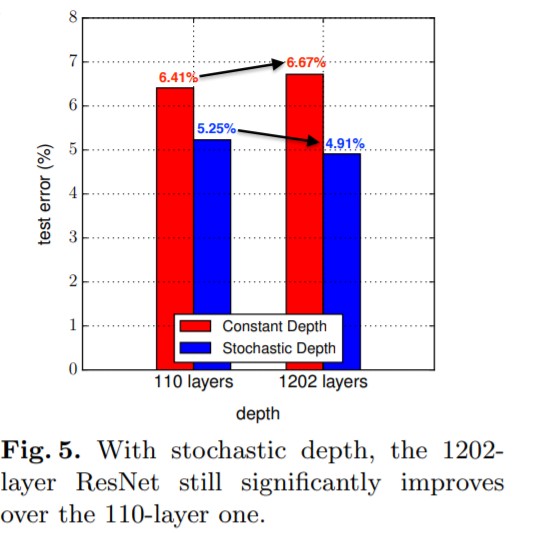
Training with a 1202-layer ResNet. He et al. [8] tried to learn CIFAR10 using an aggressively deep ResNet with 1202 layers. As expected, this extremely deep network overfitted to the training set: it ended up with a test error of 7.93%, worse than their 110- layer network. We repeat their experiment on the same 1202-layer network, with constant and stochastic depth. We train for 300 epochs, and set the learning rate to 0.01 for the first 10 epochs to “warm-up” the network and facilitate initial convergence, then restore it to 0.1, and divide it by 10 at epochs 150 and 225.
The results are summarized in Fig. 4 (right) and Fig. 5. Similar to He et al. [8], the ResNets with constant depth of 1202 layers yields a test error of 6.67%, which is worse than the 110-layer constant depth ResNet. In contrast, if trained with stochastic depth, this extremely deep ResNet performs remarkably well. We want to highlight two trends: 1) Comparing the two 1202-layer nets shows that training with stochastic depth leads to a 27% relative improvement; 2)

ImageNet.
The ILSVRC 2012 classification dataset consists of 1000 classes of images, in total 1.2 million for training, 50,000 for validation, and 100,000 for testing. Following the common practice, we only report the validation errors. We follow He et al. [8] to build a 152-layer ResNet with 50 bottleneck residual blocks. When input and output dimensions do not match, the skip connection uses a learned linear projection for the mismatching dimensions, and an identity transformation for the other dimensions. Our implementation is based on the github repository fb.resnet.torch [34], and the optimization settings are the same as theirs, except that we use a batch size of 128 instead of 256 because we can only spread a batch among 4 GPUs (instead of 8 as they did).
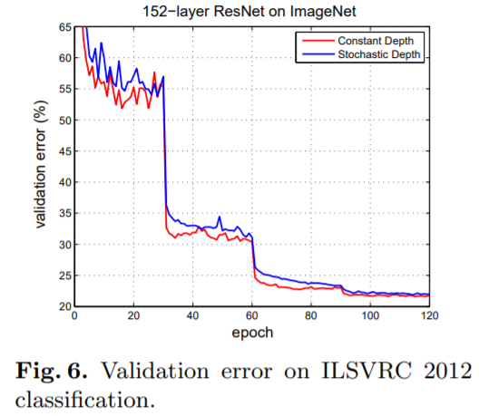
We train the constant depth baseline for 90 epochs (following He et al. and the default setting in the repository) and obtain a final error of 23.06%. With stochastic depth, we obtain an error of 23.38% at epoch 90, which is slightly higher. We observe from Fig.6 that the downward trend of the validation error with stochastic depth is still strong, and from our previous experience, could benefit from further training. Due to the 25% computational saving, we can add 30 epochs (giving 120 in total, after decreasing the learning rate to 1e-4 at epoch 90), and still finish in almost the same total time as 90 epochs of the baseline. This reaches a final error of 21.98%. We have also kept the baseline running for 30 more epochs. This reaches a final error of 21.78%.
Because ImageNet is a very complicated and large dataset, the model complexity required could potentially be much more than that of the 152-layer ResNet [35]. In the words of an anonymous reviewer, the current generation of models for ImageNet are still in a different regime from those of CIFAR. Although there seems to be no immediate benefit from applying stochastic depth on this particular architecture, it is possible that stochastic depth will lead to improvements on ImageNet with larger models, which the community might soon be able to train as GPU capacities increase.

5 Analytic Experiments
we provide more insights into stochastic depth by presenting a series of analytical results. We perform experiments to support the hypothesis that stochastic depth effectively addresses the problem of vanishing gradients in backward propagation. Moreover, we demonstrate the robustness of stochastic depth with respect to its hyper-parameter.

Fig. 7 shows the mean absolute values of the gradients. The two large drops indicated by vertical dotted lines are due to scheduled learning rate division. It can be observed that the magnitude of gradients in the network trained with stochastic depth is always larger, especially after the learning rate drops. This seems to support out claim that stochastic depth indeed significantly reduces the vanishing gradient problem, and enables the network to be trained more effectively. Another indication of the effect is in the left panel of Fig. 3, where one can observe that the test error of the ResNets with constant depth approximately plateaus after the first drop of learning rate, while stochastic depth still improves the performance even after the learning rate drops for the second time. This further supports that stochastic depth combines the benefits of shortened network during training with those of deep models at test time.


6 Conclusion In this paper we introduced deep networks with stochastic depth, a procedure to train very deep neural networks effectively and efficiently. Stochastic depth reduces the network depth during training in expectation while maintaining the full depth at testing time. Training with stochastic depth allows one to increase the depth of a network well beyond 1000 layers, and still obtain a reduction in test error. Because of its simplicity and practicality we hope that training with stochastic depth may become a new tool in the deep learning “toolbox”, and will help researchers scale their models to previously unattainable depths and capabilities.
[논문출처] : Deep Networks with Stochastic Depth
[출처]:
https://ko.wikipedia.org/wiki/%ED%96%89%EB%A0%AC%EC%8B%9D
행렬식 - 위키백과, 우리 모두의 백과사전
위키백과, 우리 모두의 백과사전. 선형대수학에서, 행렬식(行列式, 영어: determinant 디터미넌트[*])은 정사각 행렬에 스칼라를 대응시키는 함수의 하나이다.[1] 실수 정사각 행렬의 행렬식의 절댓��
ko.wikipedia.org
https://ko.wikipedia.org/wiki/%EB%B2%A0%EB%A5%B4%EB%88%84%EC%9D%B4_%EB%B6%84%ED%8F%AC
베르누이 분포 - 위키백과, 우리 모두의 백과사전
위키백과, 우리 모두의 백과사전.
ko.wikipedia.org
https://ko.wikipedia.org/wiki/%EC%BB%B4%ED%93%A8%ED%84%B0_%EB%B9%84%EC%A0%84
컴퓨터 비전 - 위키백과, 우리 모두의 백과사전
위키백과, 우리 모두의 백과사전.
ko.wikipedia.org