NAIAHD

아래 내용은 Udemy에서 Pytorch: Deep Learning and Artificial Intelligence를 보고 정리한 내용이다.

Recommender Systems with Deep Learning Theory

applicable concepts in ML

google

아마존 - Amazon

facebook

netflex

News -> exciting 한 뉴스를 본다.

Ratings Recommenders

movies

How to recommend?

Given a dataset of triples: user, item, rating

fit a model to the data: f(u, m ) ->r

what should it do?

#1. if the user u and movie m appeared in the dataset, then the predicted rating should be close to the true rating

#2. the function should predict what user u would rate movie m, even if it didn't appear in the training set

Neural networks(function approximators) do this!

since our model can predict ratings for unseen movies, this is easy 

given a user, get predicted for every unseen movie=>보지 않았든것 

Sort by predicted rating(descending)

recommend movies with the highest predicted rating

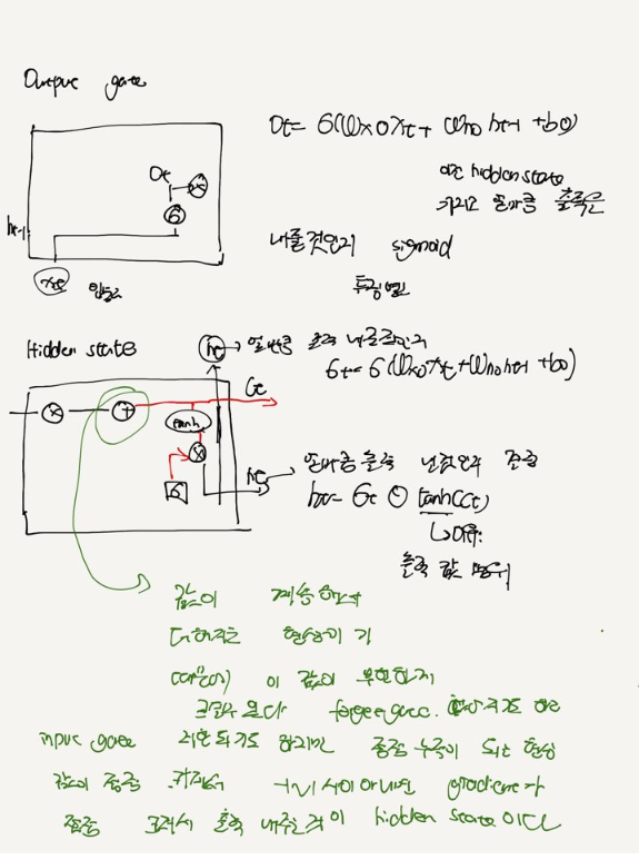
How to build the model?

users and movies categorical 

neural networks do matrix multiplications

we can't multiply a category by a number(e.g. "Start wars" x5)

NLP

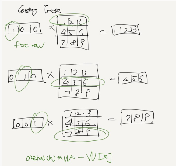
embeddings

mapping

A neural network for recommenders

Interesting point

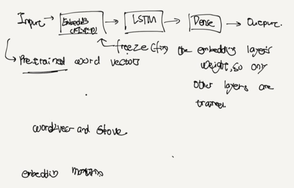
NLP 

algorithms  word2vec and GloVe

They both do things like " king-man = queen -women"

ANN  all data is the same

The inputs are clearly not an N x D matrix of features

All data is not the same

we still have N samples

1st column(users): N- length array of categories()

2nd column(movies): N- length array of categories(can bu duped)

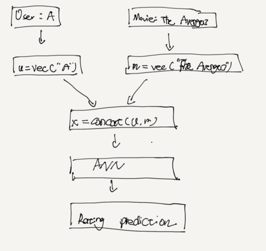
Embedding

NLP: word indexes(N x T) -> word vectors(N x T x D )

recommenders: users / movies(N) -> user/movie vectors(N x D)

How is the data stored?

They are already integers !

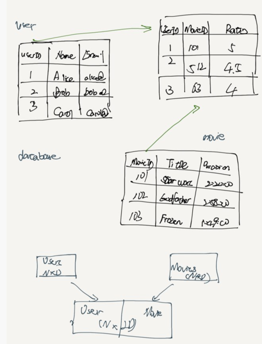
Embeddings & Concatenation

After embedding, users and movies have shape N x D

combine concatenate N x 2D

Now " all data is the same" once again

forward :

something special about this model: it has 2 inputs, not just one!

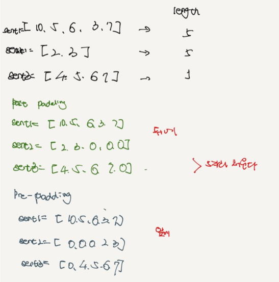
Loading in data

data is just a csv (pandas)

training 을 하기 위해서 DataLoader로 한다.

pytorch Recommender systems with deep learning code

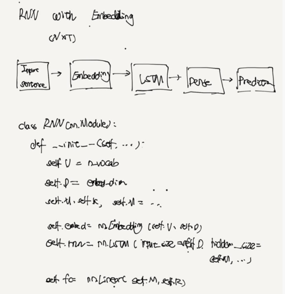
모델 만들기

class Model(nn.Module):
  def __init__(self, n_users, n_items, embed_dim, n_hidden = 1024):
    super(Model, self).__init__()
    self.N = n_users
    self.M = n_items
    self.D = embed_dim

    self.u_emb = nn.Embedding(self.N, self.D)
    self.m_emb = nn.Embedding(self.M , self.D)
    self.fc1 = nn.Linear(2 * self.D , n_hidden)
    self.fc2 = nn.Linear(n_hidden , 1)

  def forward(self, u, m ):
    u = self.u_emb(u)
    m = self.m_emb(m)

    out = torch.cat((u, m ), 1)

    out = self.fc1(out)
    out = F.relu(out)
    out = self.fc2(out)
    return out

model = Model(N, M ,D )
model.to(device)

criterion = nn.MSELoss()
optimizer = torch.optim.Adam(model.parameters())

make dataset

#make dataset
Ntrain = int(0.8 * len(ratings))
train_dataset = torch.utils.data.TensorDataset(
    user_ids_t[:Ntrain],
    movie_ids_t[:Ntrain],
    ratings_t[:Ntrain]
)

test_dataset = torch.utils.data.TensorDataset(
    user_ids_t[Ntrain:],
    movie_ids_t[Ntrain:],
    ratings_t[Ntrain:]
)

batch_size = 512
train_loader = torch.utils.data.DataLoader(dataset = train_dataset, 
                                           batch_size = batch_size,
                                           shuffle = True)

test_loader = torch.utils.data.DataLoader(dataset = test_dataset, 
                                           batch_size = batch_size,
                                           shuffle = False)

pytorch %prun 

얼마나 function에 사용했는지 알려진다.

5분 정도 걸리기 때문에 이것을 사용한다.

%prun train_losses, test_losses = batch_gd(model, criterion, optimizer, train_loader, test_loader, 25)

same prediction

pytorch weight 변경해서 하기 

class Model(nn.Module):
  def __init__(self, n_users, n_items, embed_dim, n_hidden = 1024):
    super(Model, self).__init__()
    self.N = n_users
    self.M = n_items
    self.D = embed_dim

    self.u_emb = nn.Embedding(self.N, self.D)
    self.m_emb = nn.Embedding(self.M , self.D)
    self.fc1 = nn.Linear(2 * self.D , n_hidden)
    self.fc2 = nn.Linear(n_hidden , 1)

    # set the wights since N(0,1) leads to poor results
    self.u_emb.weight.data = nn.Parameter(torch.Tensor(np.random.randn(self.N, self.D) * 0.01))
    self.m_emb.weight.data = nn.Parameter(torch.Tensor(np.random.randn(self.M, self.D) * 0.01))

  def forward(self, u, m ):
    u = self.u_emb(u)
    m = self.m_emb(m)

    out = torch.cat((u, m ), 1)

    out = self.fc1(out)
    out = F.relu(out)
    out = self.fc2(out)
    return out

device = torch.device("cuda:0" if torch.cuda.is_available() else "cpu")
model = Model(N, M ,D )
model.to(device)

criterion = nn.MSELoss()
optimizer = torch.optim.SGD(model.parameters(), lr = 0.08 , momentum = 0.9)

pytorch top 10 recommended

watched_movie_ids = df[df.new_user_id ==1].new_movie_id.values
watched_movie_ids

potential_movie_ids = df[-df.new_movie_id.isin(watched_movie_ids)].new_movie_id.unique()
print(potential_movie_ids.shape)
print(len(set(potential_movie_ids)))

user_id_to_recommend = np.ones_like(potential_movie_ids)

t_user_ids = torch.from_numpy(user_id_to_recommend).long().to(device)
t_movie_ids = torch.from_numpy(potential_movie_ids).long().to(device)

with torch.no_grad():
  predictions = model(t_user_ids, t_movie_ids)

predictions_np = predictions.cpu().numpy().flatten()
sort_idx = np.argsort(-predictions_np)

top_10_movie_ids = potential_movie_ids[sort_idx[:10]]
top_10_scores = predictions_np[sort_idx[:10]]

for movie, score in zip(top_10_movie_ids, top_10_scores):
  print("movie:", movie," score:", score)

아래 내용은 Udemy에서 Pytorch: Deep Learning and Artificial Intelligence를 보고 정리한 내용이다.

Embeddings

Text is sequence data, but it is not continuous

One-Hot Encoding?

vector  = > 0을 포함한 것 

map each word to an index 

  a => [1,0] 1

  b => [0,1] 2

T words -> one hot encoded vector of size V 

T x V matrix

data has no useful geometrical structure.

each word to a D-dimensional vector(not one-hot encoded)

RNN with Embedding

D = embedding dimension -> hypperparameter

V = vecab size (# of unique words)

Embedding matrix is V x D

Each row is a D-size vector for a word

forward Function

out = self.embed(x)

Text Preprocessing

Text Files

each word -> Integer ->vector

Structured Text Files

CSV(comma separated value)

dovument 

pandas for CSV?

document 

multiple words -> individual words

Multiple words to single words(Tokenization)

string.split() => a lot of cases

can't handle punctuation  => . 

remove 를 해야 한다. 

Tokens to Integers

dataset = long sequence of words

current_idx = 0

word2idx = {}

for word in dataset:

  if word not in word2idx :

    word2idx[word] = current_idx

    current_idx += 1

current_idx = 0 => 2로 한다. 

보통 0으로 안한다.

1 = padding

0 = unknown  => 우리는 학습을 못 할 떄 

Constant-Length Sequence

길이를 같게 하고 하기 위해 padding 을 한다.

Pre-padding vs Post-padding

- Text classification RNN reads the input from left-to-right, the pre-padding 이 더 좋다.

   시작 -> 끝 

- challenging for RNNs to learn long-term dependencies!

convert to csv

Tokenization

map each token to a unique integer

The task

text classification(many-to-one)

Input: sequence of words, output: a single label (spam or not spam)

Field Objects

import torchtext.data as ttd

TEXT = ttd.Field(

  sequentail = True,

  batch_first = True,

  lower = True,

  pad_first = True

)

LABEL = ttd.Field(sequentail = False, use_vocab = False, is_target = True)

TabularDataset Object

split train, test data

dataset.split()

build vocab

TEXT.build_vocab(train_dataset)

vocab = TEXT.vocab

vocab object

stoi(C-style naming)   문자 -> 숫자

itos(reverse mapping) 숫자 -> 문자

stoi and itos

Dictionary = keys -> values

List = keys -> value

pytorch Text Preprocessing

import torch
import torch.nn as nn
import torchtext.data as ttd
import numpy as np
import pandas as pd
import matplotlib.pyplot as plt
from datetime import datetime

data = {
    "label" : [0,1,1] ,
    "data"  :[
              "I like eggs and ham.",
              "Eggs I like!",
              "Ham and eggs or just ham?"
    ]
}
df = pd.DataFrame(data)
df.head()

df.to_csv("data.csv", index = False)

TEXT = ttd.Field(
    sequential = True,
    batch_first = True,
    lower = True,
    tokenize = 'spacy',
    pad_first = True
)

LABEL = ttd.Field(sequential=False, use_vocab=False, is_target=True)

dataset = ttd.TabularDataset(
    path = 'data.csv',
    format = 'csv',
    skip_header = True,
    fields = [('label', LABEL) ,('data' , TEXT)]
)

ex = dataset.examples[0]

train_dataset , test_dataset = dataset.split(0.66)
TEXT.build_vocab(train_dataset,)
vocab = TEXT.vocab
vocab.stoi
vocab.itos

train_iter, test_iter = ttd.Iterator.splits(
    (train_dataset, test_dataset) , sort_key = lambda x: len(x.data),
    batch_sizes = (2,2)  , device = torch.device("cuda:0" if torch.cuda.is_available() else "cpu")
)

for inputs, targets in train_iter:
  print("inputs:" , inputs, "shape:", inputs.shape)
  print("targets:" , targets, "shape:" ,targets.shape)
  break
  
for inputs, targets in test_iter:
  print("inputs:" , inputs, "shape:", inputs.shape)
  print("targets:" , targets, "shape:" ,targets.shape)
  break

CNNs for Text

sequence

1-D convolution

For images:

2 spatial dimensions + 1 input feature dimensions + 1 output feature dimension = 4

for sequences:

1 time dimension + 1 input feature dimension + 1 output feature dimension = 3

경고: feature first

Recall that for images , pytorch cnn expects image to be N x C x H x W 

  "feature first"

whereas, in Tensorflow  / OpenCV/ others, it's N x H x W x C

  "feature last"

the torchvision data generators hide this detail

NLP, output of embedding is N x T x D ("feature last")

nn.Conv1d(), we expect N x D x T as input!("feature first")

그래서 , must reshape before and after convolutions

Text Classification with CNNs

output of embediding is alwasy (N, T,D)

conv1d expects (N, D, T)

=> out.permute(0,2,1)

change it back

out.permute(0,2,1)

cnn 도 경과가 좋게 나온다.

class CNN(nn.Module):
  def __init__(self, n_vocab, embed_dim, n_outputs):
    super(CNN, self).__init__()
    self.V = n_vocab
    self.D = embed_dim
    self.K = n_outputs

    self.embed = nn.Embedding(self.V, self.D)

    self.conv1 = nn.Conv1d(self.D, 32, 3, padding = 1)
    self.pool1 = nn.MaxPool1d(2)
    self.conv2 = nn.Conv1d(32, 64, 3, padding = 1)
    self.pool2 = nn.MaxPool1d(2)
    self.conv3 = nn.Conv1d(64, 128, 3, padding = 1)

    self.fc = nn.Linear(128, self.K)
  def forward(self, X):
    out = self.embed(X)
    out = out.permute(0,2,1)
    out = self.conv1(out)
    out = F.relu(out)
    out = self.pool1(out)
    out = self.conv2(out)
    out = F.relu(out)
    out = self.pool2(out)
    out = self.conv3(out)
    out = F.relu(out)
    
    out = out.permute(0,2,1)

    out, _ = torch.max(out, 1)
    out = self.fc(out)
    return out

making predicions with Trained NLP Model

single_sentence = 'Our dating service has been asked 2 contast U by someone shy!'
toks= TEXT.preprocess(single_sentence)
sent_idx = TEXT.numericalize([toks])
model(sent_idx.to(device))

아래 내용은 Udemy에서 Pytorch: Deep Learning and Artificial Intelligence를 보고 정리한 내용이다.

GRU and LSTM

Modern RNN Units

LSTM

GRU is like 간단한 버전의 LSTM 과 비슷하다.(파라미터가 적고 thus more efficient )

simple RNN이 is not enough 는 vanishing gradient 때문이다.

 vanishing gradient해결하는데 ReLU 사용 ????????

하지만 더 효과적인 GRU, LSTM를 발견하였다.

Simple RNN은 수식이 하나이다.

GRU

recurrent Unit

SimpleRNNs have no choice bue to eventually forget, due to the vanishing gradient 

binary classifier (logistic regression neurons) as our gates 

SimpleRNN 은 long-term dependencies에 학습 할 떄 문제가 있다.

the hidden state becomes the weighted sum of the previos hidden state and new value(allowing you to remeber the old state)

these are controlled by "gates" which are like binary classifiers /logistic regression / neurons

GRU less parameter > more performent

LSTM(long-short term memory)

Simple RNN GRU LSTM code

nn.RNN(

input_size = self.D,

hidden_size = self.M,

num_layers = self.L, 

nonlinearity = 'relu',

batch_first = True

)

GRU

nn.GRU(

input_size = self.D,

hidden_size = self.M,

num_layers = self.L, 

batch_first = True

)

LSTM

nn.LSTM(

input_size = self.D,

hidden_size = self.M,

num_layers = self.L, 

batch_first = True

)

A more challenging Sequence

pytorch nonlinear sequence Linear code

import torch
import torch.nn as nn
import numpy as np
import matplotlib.pyplot as plt

series = np.sin((0.1 * np.arange(400)) ** 2)

data 만들기

T = 10
D = 1
X = []
Y = []
for t in range(len(series) - T) :
  x = series[t:t+T]
  X.append(x)
  y = series[t+T]
  Y.append(y)

X = np.array(X).reshape(-1, T)
Y = np.array(Y).reshape(-1, 1)
N = len(X)
print(X.shape, "   " , Y.shape)

model = nn.Linear(T, 1)

criterion = nn.MSELoss()
optimizer = torch.optim.Adam(model.parameters(), lr = 0.1)

train test set split

X_train = torch.from_numpy(X[:-N//2].astype(np.float32))
y_train = torch.from_numpy(Y[:-N//2].astype(np.float32))
X_test = torch.from_numpy(X[-N//2:].astype(np.float32))
y_test = torch.from_numpy(Y[-N//2:].astype(np.float32))

모델 학습 

LOSS 확인 하기

ONE-STEP forecast

validation_target = Y[-N//2:]
with torch.no_grad():
  validation_predictions = model(X_test).numpy()

Linear model has terrible result 

pytorch nonlinear sequence SimpleRNN code

T = 10
D = 1
X = []
Y = []
for t in range(len(series) - T) :
  x = series[t:t+T]
  X.append(x)
  y = series[t+T]
  Y.append(y)

X = np.array(X).reshape(-1, T , 1) #MAKE IT N x T
Y = np.array(Y).reshape(-1, 1)
N = len(X)
print(X.shape, "   " , Y.shape)

class RNN(nn.Module):
  def __init__(self, n_inputs, n_hidden, n_rnn_layers, n_outputs):
    super(RNN, self).__init__()
    self.D = n_inputs
    self.M = n_hidden
    self.K = n_rnn_layers
    self.L = n_outputs

    self.rnn = nn.RNN(
      input_size = self.D,
      hidden_size = self.M,
      num_layers = self.L,
      nonlinearity = 'relu',
      batch_first = True
    )

    self.fc = nn.Linear(self.M, self.K)

  def forward(self, X):
    
    h0 = torch.zeros(self.L, X.size(0), self.M).to(device)
    out, _ = self.rnn(X, h0)

    out = self.fc(out[:,-1,:]) 
    return out

pytorch nonlinear sequence LSTM code

class RNN(nn.Module):
  def __init__(self, n_inputs, n_hidden, n_rnn_layers, n_outputs):
    super(RNN, self).__init__()
    self.D = n_inputs
    self.M = n_hidden
    self.K = n_rnn_layers
    self.L = n_outputs

    self.rnn = nn.LSTM(
      input_size = self.D,
      hidden_size = self.M,
      num_layers = self.L,
      batch_first = True
    )

    self.fc = nn.Linear(self.M, self.K)

  def forward(self, X):
    
    h0 = torch.zeros(self.L, X.size(0), self.M).to(device)
    c0 = torch.zeros(self.L, X.size(0), self.M).to(device)
    out, _ = self.rnn(X, (h0,c0))

    out = self.fc(out[:,-1,:]) 
    return out

RNNs for Image Classification

MNIST , Fashion MNIST

H x W (2-d )

Code preparation

step 1: load in the data

step 2: model

step 3: fit / plot the loss /etc. 

regression is harder than classification

classification 은 라벨만 하면 된다.

lstm

본 내용은  fastcampus 딥러닝/인공지능 올인원 패키지 online을 정리한 것이다.

순환 신경망에서 Tensor의 이해

다양한 입력과 출력

절결합 계층의 입출력 텐서

Rnn의 입력 텐서

순차적으로 들어온다.

입력 N x L x I 입력 텐서의 앞부분을 0으로 채우는 이유는 , 마지막 입력부터는 출력이 잘 나올 수 있다.

출력 N x L x O 출력 은 뒤부분을 0으로 채운다.

순환 신경망의 학습법

BPTT: Backpropagation through time  시간 펼침 역전파

입력 N x L x I  

배치로 나눈 학습 데이터 (B x L x I)

시간적으로 펼치면서 계산해야 하는 점을 제외하면 , 보통의 역전파와 동일한다.

배치로 피우기 힘들다. 펼침을 하나씩 더해야 하기 때문에 휠씬 메모리가 필요한다.

다중 입력, 다중 출력  => Truncated BPTT데이터 입력 쪼개서 한다.

Truncated 사이에는 역전파가 이루어지지 않는다.

Rnn Embedding을 사용한다. 

몇개의 word를 사용하는지 one-hot encoding사용한다.

특정단어들이 one-hot 으로 하면 안되서 실수쪽으로 가져오기 위해서 길이가 만든 feature vector를 바꿔주는 것이다.

tensorflow IMDB data load

import tensorflow as tf
imdb = tf.keras.datasets.imdb
(X_train, y_train) ,(X_test, y_test) = imdb.load_data(num_words = 10000) # 10000 개 데이터 가져오기

# 특정 길이 짤라야 하고 앞쪽에 padding을 한다.
X_train = tf.keras.preprocessing.sequence.pad_sequences(X_train, 
                                                       value = 0,
                                                       padding ='pre',
                                                       maxlen= 32)
X_test = tf.keras.preprocessing.sequence.pad_sequences(X_test, 
                                                       value = 0,
                                                       padding ='pre',
                                                       maxlen= 32)

Attention 기법

sequence-to-sequence model => seq2seq 번역 문제를 학습히기 위해 널리 사용되고 있는 rnn구조

encoder ->context -> decoder

영어 문장의 데이터화

Tokenizer와 Embedding이 필요하다.

단어 분리  , 문장주호 제거

Tokenizer:  단어들을 숫자로 바꾼다.

Embedding :  

한글 문장의 데이터화

형태소 분석 , 문장부호 제거 가 필요하다.

Tokenizer와 Embedding이 필요하다.

RNN 문제점

Gradient Vanishing기울기 소실 : 입출력 연관 관계가 멀리 떨어져 있으면 기울기 소실이 일어나 학습이 잘 되지 않는다.

멀리 떨어지면 기울기 소실 일어난다.

-> 해결법:

전에는 context하나 전달하였지만 Encoder hidden state를 모아서 Decoder로 각각 전달하면 기울기 소실을 해결할 수있다. 새로운 context뽑아서 사용가능하다. 적은 step 타고 간다.

효율적으로 하는것이 Anttention mechanism이다. 

서로 서로 연관있게 학습니다.  어디에 집중해야 하는지 집중하는것

Attention  신경망

Query: 질의 찾고자 하는 대상

key: 키 . 저장된 데이터를 찾고자 할 때 참조하는 값

value : 값 저장되는 데이터

Dictionary : key - value pair로 이루어진 집합 쌍으로 연결 

Query 로 해서 비교 하고 값 출력한다.

Attention mechanism query key-value사용 

query key비교해서 유사한지  날리고 원하는 유사도가 높은 것을 value로 묶어서 한다.

Attention 모델에선느 key와 value를 같은 값 사용

decoder에서 찾을 려고 할때 찾을 수 있는것은 encoder단이다.

encoder layer에서 필요한 key-value encoding해서 feature vector로 가지고 있는것이기 떄문에 decoder에서 는 encoder쪽을 참조로 하겠다.

전의 hidden layer가지고 사용한다.

출력은 유사도 가 되고 value를 섞어서 결과 출력 

Attention  value 를 concatenate하여 입력한다.

Attention 

Transformer 구조 사용

Transformer 어느 위치에 사용했는지 알아야 해서 position 을 사용

RNN으로 되여있어서 순차적으로 되여있다.

병렬적으로 일어나서 조금씩 다르다.

Word Embedding

Positional Encoding: 시간적 위치별로 고유의 Code 를 생성하여 더하는 방식

위치 에 있는 것

scaled Dot - Product Attention

Query , Key Value의 구조를 띄고 있음

softmax이용

Multi-Head Attention

Linear 연산 

head를 여러개 

h개의 Attention Layer 를 병렬적으로 사용 - 더 넓은 계층

Linear하면서 차원이 줄어들었다.

Masked Multi-Head Attention

Self Attention key 와 value가 같다.

Position-wise Feed-Forward

one-hot 

단어의 개수 

단어 하나마다 입력을 여서 출력이 나온다. 병렬적으로 사용해서 

Layer normalization   : 

batch영향을 받지 않는 것 

Attention mechanism

weighted sum을 많이 사용한다.

키와 value의 쌍이 있다.

Encoder입출력

encoder 출력을 key value로 넣기

입력 sequence 길이 n 

출력 sequence 길이 m -> 언어가 달라질 수 있어서 따로 변수로 한다.

Positional Encoding 시간적 위치별로 고유의 Code를 생성하여 더하는 방식

상대적 이치가 달라진다.

동시에 계산할수 있다는 것이 병렬 연산 transformer network에 중요한 역할

konlpy -> korean nature 

pip install konlpy

Okt -> 트위트에서 만든 페키지 형태소 분석

okt.morphs()->형태소 분석

Tokenizer() -> 몇개까지 fitting을 해준다.

각 단어들을 숫자로

ground truth -> test의 정답

과적합의 해결

overfitting 너무 과하게 fitting 

학습 데이터에 너무 fitting되여 있어서 test데이터에 성능이 떨어진다.

dataset

train data : 모델 학습 

validation data : 학습이 잘 되는지 검증

test data : 학습이 끝난후 모델 평가 -> 공정하게 하는 것 

1. early stopping: 감소하지 않으면 중단한다.

2. droup out : fully connect에서 몇개 제거하는 방법

3. Batch Normalization 

정규화 기법 Regularization:

알고리즘의 일반화 Generalization 를 개선하려는 모든 기법

정규화 기법을 도입하면서 loss값이 감소하는 것을 기대하면 안된다. => loss값을 증가하는 추세가 보인다.

loss training 에서 감소하지 않아도 validation에서 감소하는 목적을 하기 위하여 

흔히 최적화에 추가적인 손실 함수를 추가하는 것을 정규화 기법이라 부른다.

Weight Decay

 Weight의 l-2 Norm 을 최소화하는 정규화 기법, Weight가 지나치게 커지는 것을 막는다.

영상 복원문제 

VGG Loss : Vgg 16의 Feature만 사용

SSIM 화질 평가 기법 Structural Similarity Index

본 내용은  fastcampus 딥러닝/인공지능 올인원 패키지 online을 정리한 것이다.

WARNING:

tensorflow:Layer mymodel_2 is casting an input tensor from dtype float64 to the layer's dtype of float32, which is new behavior in TensorFlow 2. The layer has dtype float32 because its dtype defaults to floatx. If you intended to run this layer in float32, you can safely ignore this warning. If in doubt, this warning is likely only an issue if you are porting a TensorFlow 1.X model to TensorFlow 2. To change all layers to have dtype float64 by default, call `tf.keras.backend.set_floatx('float64')`. To change just this layer, pass dtype='float64' to the layer constructor. If you are the author of this layer, you can disable autocasting by passing autocast=False to the base Layer constructor.

해결방법:

X_train= X_train[..., tf.newaxis].astype(np.float32)
X_test= X_test[..., tf.newaxis].astype(np.float32)

Residual Unit 개발 주의 할점

Pre-Active

batch normalization  ->relu -> conv

채널 개수 같아야 한다.

학습 할때는 training = True

test할 떄는 training = False

DenseNet 개발 주의 할점

concatenate

concatenate([input, batch normalization ->relu -> conv ])

growth rate

학습 할때는 training = True

test할 떄는 training = False

순차 데이터의 이해

순서가 의미가 있으며, 순서가 달라질 경우 의미가 손상되는 데이터를 순차 데이터라고 한다.

Resampling  : 일정한 간격으로 다시 samping해주면

심층 신경망과 순차 데이터

다중 입력, 단일 출력

다중 입력, 다중 출력

단일 입력, 다중 출력

Memory System => 그 전의 내용을 기억해야 한다.

Memoryless System 무기억 시스템 :

  shallow neural network 이전 입력에 영향을 받지 않는다. 출력에도 영향을 받지 않는다.

vanilla Recurrent Network: 기본적인 순환 신경망 

얕은 신경망 구조에 '순환'이 추가된 것으로 

이전의 모든 입력에 영향을 받는다.

기울기 소실 문제 때문에 잘 사용하지 않는다.

multi-layer RNN: 다중 계층 순환 신경망

권장되는 구조는 아니다. 학습이 잘 되지 않는다.

LSTM LONG Short-Term Memory

필요한 시간 만큼 기억한다.

Cell State가 추가 됬다. -> 오래동안 기억을 잘 하기 위해서  덧셈

Hidden State -> 출력 

Forget Gate -> sigmoid로  얼만큼 잊을 지 결정

 0 이 곱해진것은 잊어버리고 1곱한것은 남는다.

Input Gate  -> sigmoid 새롭게 추출한 특징을 얼만큼 사용할 지 결정

  얼마큼 기억할 것인지

Output Gate -> sigmoid Cell 로부터 출력을 얼마나 내보낼지 결정 

GRU Gated Recurrent Unit

 LSTM을 간소화한 버전 

Cell state가 없고, hidden state만 존재

Forget Gate와 Input Gate합쳐졌다.  -> Forget Gate를 사용 

 잊은것을 채워주는  기억을 어떻게 할것인지

Reset Gate sigmoid 곱해진다. 새로운 Feature를 뽑기전에 기억을 얼마나 죽여줄지 

순환 신경망은 기본 역전파 학습법으로는 학습할 수없다.

순차 데이터셋의 구조

순차 데이터 -> 순환 신경망

순방향 추론  : 입력을 여러번 해주면 마지막 출력이 나온다.

시간 펼침 역전파 Back Propagation Through Time

사이의 미분을 다 알아야 한다.

시간적으로 펼쳐진 변수들은 동일한 변수라는 점에 유의해야 한다.

All -Zero 입력

LSTM LONG Short-Term Memory

Cell state, hidden state, forget gate, input gate, output gate , hidden state
forget gate input gate Cell state output gate hidden state

forget gate 기억을 '잊고자 하는 정도'를 나타낸다. 

simoid activation 이므로 값의 범위는 0~1이다.

특징별로 기억할지 말지를 결정할 수 있다.

input gate : 새로운 입력을 받고자 하는 정도를 나타낸다. sigmoid activation 이므로 값의 범위는 0~ 1이다.

특징은 여러 차원으로 되어있으므로 , 특징별로 받아들일지 말지를 결정할 수 있다.

Cell state '기억'을 총괄하는 메모리 역할을한다. 여러 차원으로 되어있어 , 각차원은 특정 정보를 기억한다.

hadamard연산자의 특성으로 인해 , 특징 별로 기억하고 , 잊고 ,새로이 정보를 받을 수 있다.

output gate 는 cell state중 어떤 특징을 출력할지 결정하는 역할을 한다. sigmoid

hidden state Cell state에 tanh activation을 적용한 후, output gate로 선별하여 출력한다.

tanh -1~1로 bound되게 하기 위함이다.

GRU수식

Reset gate  forget gate hidden state

Reset gate :  hidden state중 어떤 특징을 reset할지 결정한다.

forget처럼 바로 잊어버리는것이 아니고 

기억을 해야 하지만 큰 맥락에서는 feature를 뽑는 방해가 되는것이 있을 수 있다.

forget gate: 이전 time 의 hidden state를 잊어버린다 . 1- 에서 빼준다.

hidden state: 이전 reset gate,forget gate를 모두 적용하여 hidden state를 계산한다. 

제어가 된만큼 넘어오고 입력과 이전 time의 reset gate를 정의해서 reset gate에의해서전에것

잊어버리고 다시 한다.

계속 누적해서가 아니고 이전의 잊어버린 만큼만 하기 때문에 tanh가 필요없다.

본 내용은  fastcampus 딥러닝/인공지능 올인원 패키지 online을 정리한 것이다.

의존성이 있는 함수의 계산:

서로 서로 계산에 관계가 있다.

단점은 : 중복되는 연산이 있을 수 있다.

동적 계획법 : Dynamic Programming -> 알고리즘

첫 계산시 값을 저장하므로 중복 계산이 발생하지 않는다. 

나중에 사용할 것을 미리 저장하고 나중에 사용한다.

피보나치 계산 등 동벅 계획법을 사용하였다.

Recursion(재귀)  

연쇄 법칙 Chain Rule:

연속된 두 함수의 미분은, 각 함수의 미분을 연쇄적으로 곱한 것과 같다. 

심층 신경망의 미분: 연쇄 법칙을 이용하려면 손실 함수의 미분이 필요하다.

저장해 두었다가 중복 연산을 피할 수 있다.

앞쪽으로 미분을 계산하는 것이 역전파 학습 법 : Back-Propagation

블랙박스 모델의 학습:

학습 목표 : 손실 함수를 최소화 하는 매개변수를 찾는다.

수치적 기울기:  각 스칼라 변수를 각각 조금씩 바꾸어 대입해 보면서 수치적 기울기를 구한다.

fully connect layer:

sigmoid 함수의 미분: 

역전파 알고리즘: BP

수치미분

python 환경설정

anaconda 로 설치 -window

www.anaconda.com/products/individual#windows

설치 

jupyter notebook Launch 한다.

New => Python로 해서 새로운 파일 생성한다.

파일이 녹색으로 되여있으면 실행중 이다.

합성공 연산과 이미지 필터

아날로그 신호처리

LTI 시스템은 선형적이고 시간의 영향을 받지 않는다.

사람은 LTI시스템이 아니다.

Dirac 델타 함수 

임펄스 응답 : -> filter

Convolution  

함수 두개를 합성해서 곱한다.

두 함수의 곱을 적분하여 계산

겹치는 부분에 적분을 한다.

잡음 제거 필터

2차원 신호 

흑백 영상은 각 픽셀이 0~1 사이의 실수로 된 2-D 신호로 표현할 수 있다.

컬러 영상은 RGB 3채널로 구성된 2-D 신호로 표현할 수있다.

합성곱 계산

양상과 겹치는 부분을 곱한다.

잡음 제거 필터 :

가우시안 

미분 필터 

뉴런: Nureon

input 

weight

bias 

Convolutional layer

의미: '특징' 이 나타나는 위치를 찾아내는 것이 다.

특정 위치의 값을 크게 해주는 것이다.

pooling layer: 영상의 크기가 줄어들고 , 정보가 종합된다.

average, max

flatten  : 아무런 연산도 안일어난다고 생각하면 된다.

fully connected layer: 추출한 특징을 얕은 신경망을 사용하는 것과 동일하다.

Receptive Field: input 영상이 있을 경우 얼마만큼 차지하는 범위

LeNet - 5 : 98년도 

VGG-16: 2014년도 

Convolutional layer

Feature map

padding

zero-padding

stride 하나씩 거너뛰여서 한다. 출력의 크기가 줄어든다.

pooling

배치 정규화 

vanilla gradient descent 

stochastic gradient descent SGD: 

gradeint 를 한번 업데이트 하기 위해 일부의 데이터만을 사용한다.

mini batch 학습법

학습데이터 전체를 한번 학습하는 것을 epoch

한번 gradient를 구하는 단위를 batch라고 한다.

Internal Covariate shift

Batch Normalization : 정규분포 

Training Phase:

학습 단계에서 들어갔을 경우 , 정규화를 한다. 

각 배치별로 계산 

Batch Normalization -> Relu하면 0아래 다 날라서  그래서 결정 해주는 것이 있다. 

Batch Normalization로 인해 , 모든 계층의 Feature 가 동일한 Scale이 되어 학습를 경쟁에 유리하다.

추론 단계 Inference Phase:

training 으로 아니면 test로 하는지 

합성공 신경망 역사 

GoogLeNet(Inception) -> 복잡하다.

Inception 모듈

 다양한 feature를 나누어서 학습한다.

 Bolleneck구조 : 연산량을 줄이기 위해 1x1 합성곱 계층. 이러한 구조  줄어든 개수의 영역 

   연산량을 줄인다.

 Receptive field를 유지하면서 파라미터의 수와 연산량을 줄였다.

파라미터 수 줄이는것은 연산량을 줄이는 것과 같다.

추가적으로 분류기 달아서 기울기 소실 문제 해결한다.

Residual Network

Facebook에서 딥러닝 네트워크

152 layer

skip-connectin :  Feature 를 추출하기 전후 더한다.

Identity Mapping: 

Pre-activation

Densely Connected ConvNets DenseNet

중간중간에 Dense를 하나 추가한다.

ResNet의 아이디어를 계승하여 

Dense Block 

Growth Rate  = 4 => 4만큼의 feature를 만든다.

Bottleneck구조 :  급격하기 증가하는 것을 막기 이해 , 연산량을 줄인다.

본 내용은  fastcampus 딥러닝/인공지능 올인원 패키지 online을 정리한 것이다.

딥러닝 관련 개념

인공지능: 기계가 사람의 행동을 모방하게 하는 기술

기계학습: 기계가 일일이 코드로 명시하지 않은 동작을 데이터로부터 학습 하여 실행할 수 있도록 하는 알고리즘을 개발하는 연구 분야

딥러닝: 기계학습의 한 분야인 인공 신경망에 기반하여 , 많은 양의 데이터를 학습해 뛰어난 성능을 이끌어내는 연구 분야  => 인공신경망

빅데이터 : 인공지능, 기계학습 , 딥러닝 걸쳐 있다. 

딥러닝:

특징 추출 Feature Extraction

특징 백터

Classification

Regression

Object Detection

Image Segmentation

Image Super Resolution

Reinforcement Learning

기울기 소실 문제 로 두번째 AI Winter

깊이 깊을 수록 기울기 소실 문제 가 생긴다.

DBN : Deep Belief Network

신경망

신경 세포 : 

shallow Neural Network

인공신경망  : 뉴런이 모여 서로 연결된 형태

fully - connected  layer -> Dense Layer

얕은 신경망 : 입력, 은닉, 출력의 3가지 계층으로 

회귀 : 잡음이 있는 학습 샘플로부터 규칙을 찾아 연속된 값을 찾아가는 것 

분류 : 특정 범주로 구분하는 작업

입력 계층은 아무런 연산도 일어나지 않는다.

계층의 크기 = Node의 개수 = 입력 Scalar의 수 = 입력 Vector의 길이

단순 선형 회귀: Linear regression:

데이터를 가장 잘 표현하는 선형식을 찾는 동작

평균 제곱 오차 : Mean Squared Error

y = [10.5, 3.6]

y= [8.3, 4.6]

 => E = (10.5 - 8.3 ) ^2 + (3.6 - 3.8) ^

 = 5.8

이진 분류 문제

잘 끝는 선이 Decision Boundary

sigmoid function => 이진 분류 문제 , 확률

값이 작을 수록 0 , 커질 수록 1에 수렴

모든 실수 입력 값에 대해 출력이 정의됨

모든 점에서 미분 가능

입력 값이 0에 가까울 수록 출력이 빠르게 변함

확률 표현

교차 엔트로피 오차 Cross entropy error : CEE

틀릴 수록 오차가 무한히 증가하는 특징이다.

Multi-class Classification:

어떤 문제인지 표현

one-hot Encoding: 한개의 값만 1이고, 나머지 값은 0으로 표현한느 기법

index elementery가 의미가 있다.

sigmoid vs. softmax

sigmoid는 2가지 클래스를 구분하기 위해 1개의 입력을 받는다.

softmax는 여러개 분류

교차 엔트로피 오차

오차를 내는 과정에서는 정답 클래스만 비교하지만, 다중 클래스 분류의 활성화함수인 softmax로 인해 다른 클래스에 대한 학습에도 영향을 준다.

sigmoid:

def sigmoid(x):
    return 1 / (1 +np.exp(-x))

softmax:

def sofmax(x):
    e_x = np.exp(x)
    return e_x / np.sum(e_x)

지고 학습: 라벨이 되여있다.

학습 매개변수 : 학습 과정에서 값이 변화하는 매개변수 , 이 값이 변화하면 알고리즘 출력이 변화

손실함수: 알고리즘이 얼마나 잘못하고 있는지를 표현하는 지표

경사하강 학습법 :

최적화

손실함수를 최소로 하는 입력값(최적값)을 찾아내는 연구 

Brute-Force: 무차별 대입법

가능한 모든 수를 대입해 보는 방법

경사는 기울기(미분, Gradient)를 이용해 계산한다.

볼록 함수 Convex Function: 어디서 시작하더라도 경사 하강법으로 최적 값에 도달 할 수 있다.

분석적 방법: 함수의 모든 구간을 수식으로 알 때 사용하는 수식적인 해석 방법

수치적 방법: 함수의 형태와 수식을 알지 못할 때 사용하는 계산적인 해석 방법

기울기는 스칼라를 백터로 미분한 것이며 , 벡터의 각 요소로 미분하면 된다.

비볼록 함수 : Non-convex Function

안전점 saddle point은 기울기가 0이 되지만 극값이 아닌 지점을 말한다.

관성 momentum:  local minimum과 잡음에 대처할 수있다.

이전 기울기에 영향을 받도록 하는 방법

속도를 기억하면서 관성 계수를 곱해서 다음에 영향을 준다.

이동 vecotr를 추가로 기억해야 해서 메모리 2배 

AdaGrad: 변수별로 학습률ㄹ이 달라지게 조절하는 알고리즘

계속 누적해서 커져서 학습이 오래 진행되면 더 이상 학습이 이루어지지 않는 단점이 있다.

한번 커지면 줄어지지 않는다. 

그래서 RMSProp : AdaGrad의 문제점을 개선한 방법으로 , 합 대신 지수 평균을 사용

Adam: Adaptive moment estimation: RMSProp 과 Momentum 의 장점을 결합한 알고리즘

Adam최적화 방법은 sota 이며 , 딥러닝에서 가장 많이 사용된다.

shallow Neural Network:

가장 단순하고 얕은 (은닉 계층이 하나) 인 구조

Deep Nerual Network:

보통 layer가 5개 이상 

은닉 계층 추가 = 특징의 비선형 변환 추가

입력을 추가하면서 점점 linear하게 생긴다.

학습 매개변수의 수가 계층 크기의 제곱에 빌{

sigmoid활성 함수 동작이 원할하지 않음 =>ReLU 도입 필요

본 내용은  fastcampus 딥러닝/인공지능 올인원 패키지 online을 정리한 것이다.

pytorch seed

torch.manual_seed(seed)

tensorflow

(28,28,1)

pytorch

(1,28,28)

np.argmax() => 최대로 보여주기

전처리 함수

torchvision으로 전처리 한다.

image = Image.open(path)

np.array(image).shape

pytorch image preprocessing

중간으로 짜르기

torchvision.transforms.CenterCrop(size = (300,300))(image)

ColorJitter

FiveCrop  => 5개 모양으로 바꿔진다. list형태로 

Grayscale =>grayscale로 바꾸기

Pad( ) =>padding추가 가능

RandomApply() => 비율로 한다.

RandomChoice() => 위의 것을 random하게 선택

RandomCrop() =>자동으로 crop한다.

RandomGrayscale() => random하게 가져온다.

RandomHorizontalFlip() =>random으로 한다.

Resize() => resize해준다.  처음 부터 다르면 input안되서 resize해주고 하는것이 좋다.

RandomErasing() =>없에기

transpose(1,2,0) => plt사용할 경우