아래 내용은 Udemy에서 Pytorch: Deep Learning and Artificial Intelligence를 보고 정리한 내용이다.
7. what is machine learning?
machine learning 이란?
복잡
machine learning is nothing but a geometry problem
regression number
fit a line or curve
예측
y hat = mx + b
make the line/curve close to the data points
classification category/label
target
separate
make the line/curve separate data points of different classes
supervised learning
8. regression basics
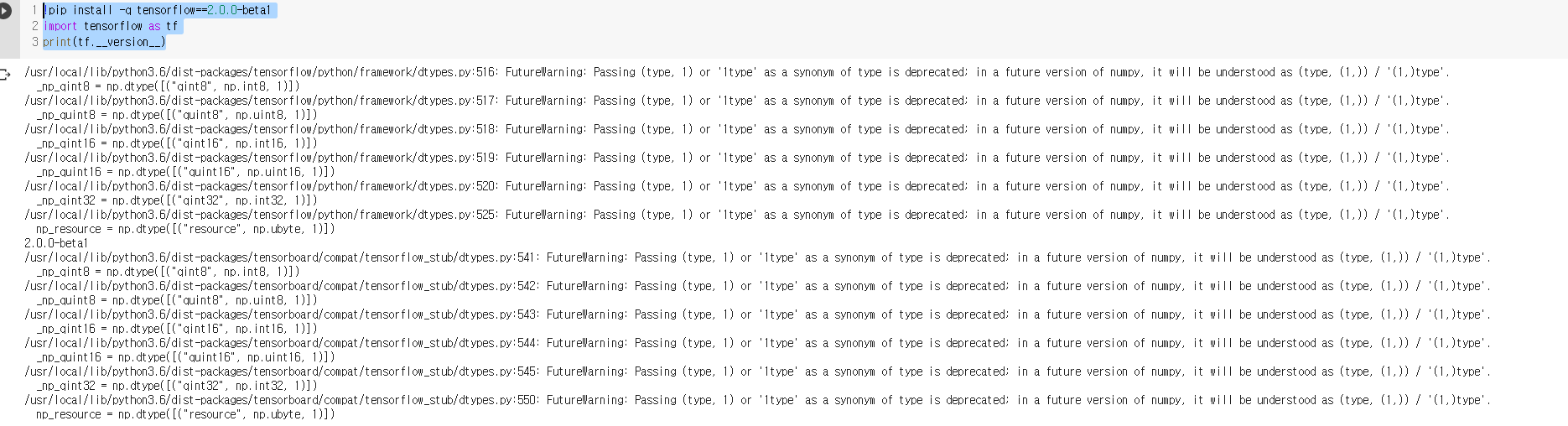
tensorflow
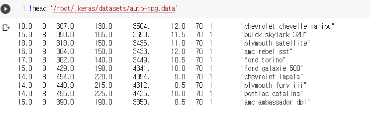
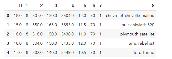
dataset
x-axis
y-axis
scikit-learn approach
load the data => pd.read_csv()
1. model architecture model = LinearRegression()
2. model.predict(X)
3. model.fit(X, y)
loss function
loss = cost == error = objective
pytorch 다른점
no predefined models
no fit or predict
mse loss 함수
Mean Squared Error : 차이
error가 작으면 작을 수록 good fit이고
크면 bad fit
perfect fit = zero error
linear regression
gradient descent
9. Regression Code Preparation
Regression code preparation
cocepts는 같지만 코드는 다르다.
python loop
for i in range(10):
print(i)
java loop
for(int i = 0; i < 10; i++){
System.out.println(i);
}
we konw the concepts, but not the syntax
#1. build the model
model = nn.Linear(1,1)
#2. train the model
#loss and optimizer
criterion = nn.MSELoss()
optimizer = torch.optim.SGD(model.parameters(), lr=0.1)
#Train the model(gradient descent loop)
n_epochs = 30
for it in range(n_epochs):
# zero the parameter gradients
optimizer.zero_grad()
# gradient
# forward pass
outputs= model(inputs)
loss = criterion(outputs, targets)
# backward and optimize
loss.backward()
optimizer.step()
(inputs, targets)
(X, y)
pytorch에서 numpy 는 안된다. tensor은 된다.
Array to tensor
X = X.reshape(N,1)
Y = Y.reshape(N,1)
#pytorch는 type에 엄청 까다롭다.
#pytorch는 float32 default
#numpy float64 default
inputs = torch.from_numpy(X.astype(np.float32))
targets = torch.from_numpy(Y.astype(np.float32)
#3. make predictions
#Forward pass
outpus = model(inputs)
<- No, this just gives us a Torch Tensor
pytorch는 tensor 가능하다.
predictions = model(inputs).detach().numpy()
<-Detach from graph(more detail later), and convert to Numpy array
summary:
10. Regression Notebook
import torch
import torch.nn as nn
import numpy as np
import matplotlib.pyplot as plt
N = 20
X= np.random.random(N) * 10 -5
y = 0.5 * X - 1 +np.random.randn(N)plt.scatter(X,y )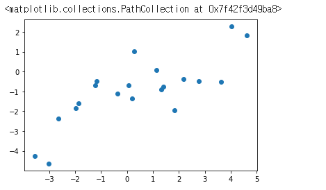
linear one input one output
model = nn.Linear(1,1)criterion = nn.MSELoss()
optimizer = torch.optim.SGD(model.parameters(), lr=0.1)X = X.reshape(N, 1)
y = y.reshape(N, 1)
inputs = torch.from_numpy(X.astype(np.float32))
targets = torch.from_numpy(y.astype(np.float32))type(inputs)torch.Tensor =>torch.Tensor
n_epochs = 30
losses = []
for it in range(n_epochs):

  optimizer.zero_grad()

  outputs= model(inputs)
  loss = criterion(outputs, targets)

  losses.append(loss.item())

  loss.backward()
  optimizer.step()

  print(f'Epoch {it+1}/{n_epochs}, Loss:{loss.item():.4f}')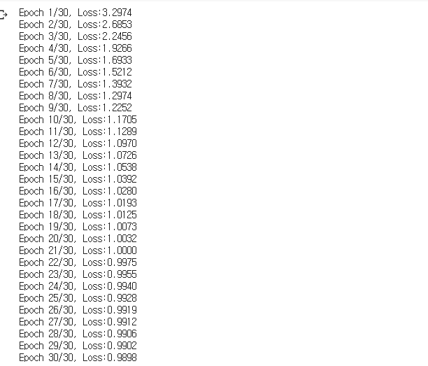
plt.plot(losses)
prediction
predicted = model(inputs).detach().numpy()
plt.scatter(X, y , label ='Original data')
plt.plot(X, predicted, label ='Fitted lne')
plt.legend()
plt.show()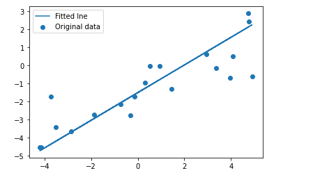
#Error
model(inputs).numpy()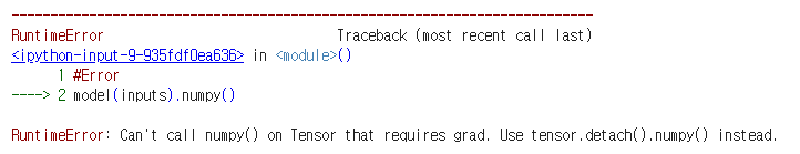
with torch.no_grad():
  output = model(inputs).numpy()
output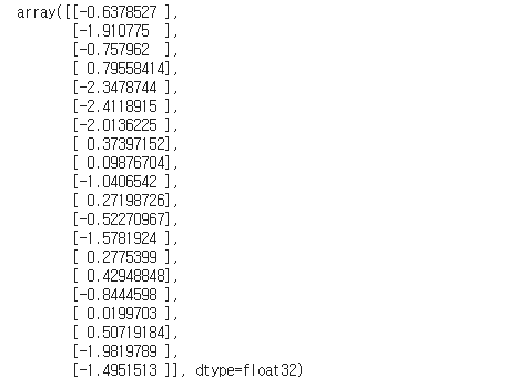
w = model.weight.data.numpy()
b = model.bias.data.numpy()
print(w, b)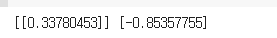
11. 무어의 법칙
무어의 법칙은 컴퓨터구조에서 배운다.
컴퓨터 power 은 grows exponentially.
2배씩
computer power
exponentailly eg, 1,2,4,8,...
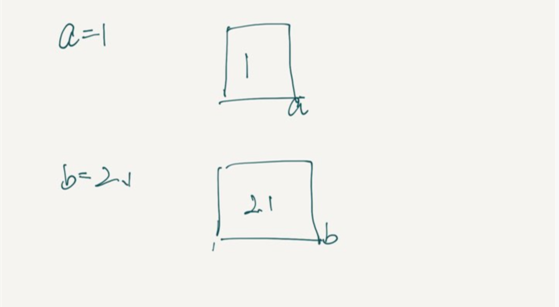
y = ax+ b=> linear 함수
normalize
12. Moore's Law Notebook
데이터를
Error tokenizing data 오류가 날 경우에는
error_bad_lines=False 추가한다.
데이터가 바꿔져서 그런지 오류가 나서 진행이 안된다.
데이터 가공
모델 생성
loss
모델 학습
모델 predict
transforming back to original scale
import torch
import torch.nn as nn
import pandas as pd
import numpy as np
import matplotlib.pyplot as plt
data = pd.read_csv('moore.csv' , header= None , error_bad_lines=False).values
data
13. Linear Classification Basics
regression: we want the line to be close to the data points
classification : we want the line to separate data points
| tensorflow 모델 학습 | pytorch | |
| 1. load in some data | ||
| 2. model 생성 | model = MyLinearClassifier() | |
| 3. train model | model.fit(X,y) | 없다. |
| 4. predictions | model.predict(X_test) | 없다. |
| 5. evaluate accuracy | model.score(X,y) |
accuracy = #correct / #total
error = #incorrect/ #total
error = 1- accuracy
linear
a = w1x1+w2x2 +b
if a>= 0 -> predict 1
if a< 0 -> predict 0
sigmoid 0 ~ 1 사이의 값
model architecture
making predictions
training
14. Classification Code Prepatration
loading in the data
from sklearn.datasets import load_breast_cancer

data = load_breast_cancer()
X,y = data.data, data.target
preprocess the data
split the data
from sklearn.model_selection import train_test_split
from sklearn.preprocessing import StandardScaler

X_train, X_test, y_train, y_test = train_test_split(X, y, test_size =0.3)
scaler = StandardScaler()
X_train = scaler.fit_transform(X_train)
X_test = scaler.transform(X_test)
build the model
Recall: the shape of the data is "NxD"
model = nn.Sequentail(
nn.Linear(D,1),
nn.Sigmoid()
)
input each feature for dataset
Train the model
#loss and optimizer
criterion = nn.BCELoss() #binary cross entropy
optimizer = torch.optim.Adam(model.parameters()) #adam hypperparammeter
for it in range(n_epochs):
optimizer.zero_grad()
hypperparameter
evaluating the model
Recall : in regression , we use the MSE(loss)
RMSE 도 가능하다.
GET THE ACCURACY:
with torch.no_grad():
p_train = model(X_train)
p_train = np.round(p_train.numpy())
train_acc = np.mean(y_train.numpy() == p_train)
15. Classification Notebook
pytorch Classification code
import torch
import torch.nn as nn
import numpy as np
import matplotlib.pyplot as plt
from sklearn.datasets import load_breast_cancer
data = load_breast_cancer()
type(data)
data.keys()
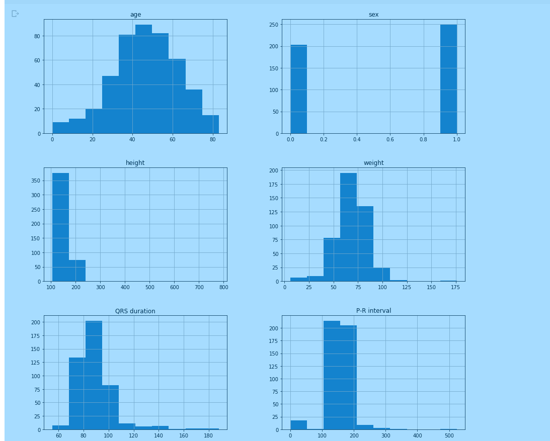
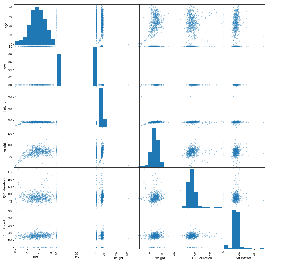
shape를 확인한다.
data.data.shape

569 데이타 가 있고 30개 feature이 있다.
data.target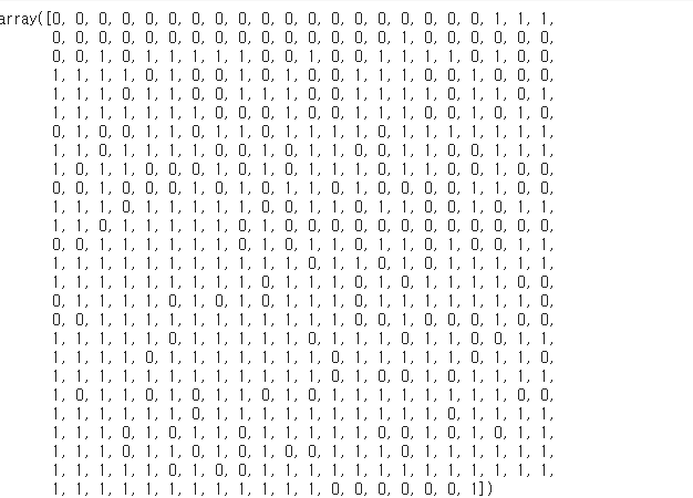
data.target_names
data.target.shape
data.feature_names
data split
from sklearn.model_selection import train_test_split
X_train, X_test, y_train, y_test = train_test_split(data.data, data.target, test_size =0.3)
N, D = X_train.shape
normalization or standardscaler
from sklearn.preprocessing import StandardScaler


scaler = StandardScaler()
X_train = scaler.fit_transform(X_train)
X_test = scaler.transform(X_test)
pytorch build model
model = nn.Sequential(
  nn.Linear(D,1),
  nn.Sigmoid()
)
loss and optimizer
criterion = nn.BCELoss()
optimizer = torch.optim.Adam(model.parameters())
convert data tensor
2d array -> 1d array
X_train = torch.from_numpy(X_train.astype(np.float32))
X_test = torch.from_numpy(X_test.astype(np.float32))
y_train = torch.from_numpy(y_train.astype(np.float32).reshape(-1,1))
y_test = torch.from_numpy(y_test.astype(np.float32).reshape(-1,1))
epochs = 1000
train_losses = np.zeros(epochs)
test_losses = np.zeros(epochs)
for epoch in range(epochs):
optimizer.zero_grad()
outputs = model(X_train)
loss = criterion(outputs, y_train )
outputs_test = model(X_test)
loss_test = criterion(outputs_test, y_test)
#save losses
train_losses[epoch] = loss.item()
test_losses[epoch] = loss_test.item()
if (epoch+1) % 50 == 0:
print(f'Epoch {epoch+1}/ {epochs} , Train loss: {loss.item():.4f} , Test loss: {loss_test.item():.4f}' )
plt.plot(train_losses , label = 'train loss')
plt.plot(test_losses , label = 'test loss')
plt.legend()
plt.show()
#loss function
accuracy
# get Accuracy
with torch.no_grad():
  p_train = model(X_train)
  p_train = np.round(p_train.numpy())
  train_acc = np.mean(y_train.numpy() == p_train)

  p_test = model(X_test)
  p_test = np.round(p_test.numpy())
  test_acc = np.mean(y_test.numpy() == p_test)

print(f"Train acc: {train_acc:.4f} , Test acc:{test_acc:.4f}")
loss and accuracy
plt.plot(train_acc , label = 'train acc')
plt.plot(test_acc , label = 'test acc')
plt.legend()
plt.show()
16. Saving and loading a model
pytorch saving and loading model
dictionary
model.state_dict()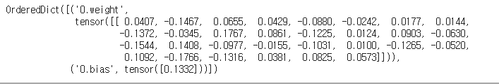
save the model
torch.save(model.state_dict(), 'myFirstModel.pt')!ls
model1 = nn.Sequential(
  nn.Linear(D,1),
  nn.Sigmoid()
)
model1.load_state_dict(torch.load('myFirstModel.pt'))
# get Accuracy
with torch.no_grad():
  p_train = model1(X_train)
  p_train = np.round(p_train.numpy())
  train_acc = np.mean(y_train.numpy() == p_train)

  p_test = model1(X_test)
  p_test = np.round(p_test.numpy())
  test_acc = np.mean(y_test.numpy() == p_test)

print(f"Train acc: {train_acc:.4f} , Test acc:{test_acc:.4f}")
google colab 모델 다운로드 하기
from google.colab import files
files.download('myFirstModel.pt')
구글에서 다운로드가 된다.
17. A short Neuroscience Primer
linear regression y = ax + b
logistic regression
nueron network
nueron
senses -> signals
18. How does a model "learn"?
linear regression
line of best fit
mse mean squared error
minimizing cost -> making small is possible
gradient ->기울기
gradient Descent
gradient zero
epochs to train
gradient Descent
learning rate -> hyperparameter
19. Model With logits
전 부 같은데 모델 생성하는 부분이 다르다.
계산이 포함 되여 있어서 sigmoid 필요없다.
model2 = nn.Linear(D,1)

criterion = nn.BCELoss()
optimizer = torch.optim.Adam(model2.parameters())
prediction 도 다르다.
숫자로 결과를 나오기 때문에 확인 해야 한다.
# get Accuracy
with torch.no_grad():
  p_train = model2(X_train)
  p_train = np.round(p_train.numpy() > 0)
  train_acc = np.mean(y_train.numpy() == p_train)

  p_test = model2(X_test)
  p_test = np.round(p_test.numpy() > 0)
  test_acc = np.mean(y_test.numpy() == p_test)

print(f"Train acc: {train_acc:.4f} , Test acc:{test_acc:.4f}")
20 Train Sets vs. Validation Sets vs. Test Sets
overfitting을 방지하기 위하여 데이터 셋을 나눈다.
optimim 찾기
cross-validation
hypperparameter
21. Suggestion Box
'교육동영상 > 02. pytorch: Deep Learning' 카테고리의 다른 글
| 06-2. Recurrent Neural Networks, Time Series, and Sequence Data (0) | 2020.12.14 |
|---|---|
| 06. Recurrent Neural Networks, Time Series, and Sequence Data (0) | 2020.11.20 |
| 05. Convolutional Nerual Networks (0) | 2020.11.19 |
| 04. Feedforward Artificial Neural Networks (1) | 2020.11.18 |
| 01. Introduction 02. Google Colab (0) | 2020.11.14 |