반응형

본 내용은  fastcampus 딥러닝/인공지능 올인원 패키지 online을 정리한 것이다.


이미지 전처리

augmentation


python glob # 경로 너주면 한번에 읽어오기 

os.lisdir() 과 glob차이 :

os.listdir() => 하위에 있는 파일 다 읽어 온다.  파일 명만 가져온다.

glob.glob() => 필요한 파일 가져올 수 있다.


데이터 분석


How to download MNIST images as PNGs?

import gzip
f = gzip.open('./dataset/MNIST/raw/train-images-idx3-ubyte.gz','r')

image_size = 28
num_images = 5

import numpy as np
import matplotlib.pyplot as plt

f.read(16)
buf = f.read(image_size * image_size * num_images)
data = np.frombuffer(buf, dtype=np.uint8).astype(np.float32)
data = data.reshape(num_images, image_size, image_size, 1)
image = np.asarray(data[2]).squeeze()
plt.imshow(image)


stackoverflow.com/questions/55049511/how-to-download-mnist-images-as-pngs


How to download MNIST images as PNGs

I want to download the MNIST images to my computer as PNG files. I found this page: http://yann.lecun.com/exdb/mnist/ After I pressed: train-images-idx3-ubyte.gz: training set images (9912422 bytes)

stackoverflow.com

github.com/myleott/mnist_png/blob/master/convert_mnist_to_png.py


myleott/mnist_png

MNIST converted to PNG format. Contribute to myleott/mnist_png development by creating an account on GitHub.

github.com


import os
import struct
import sys

from array import array
from os import path

import png

# source: http://abel.ee.ucla.edu/cvxopt/_downloads/mnist.py
def read(dataset = "training", path = "."):
    if dataset is "training":
        fname_img = os.path.join(path, 'train-images-idx3-ubyte')
        fname_lbl = os.path.join(path, 'train-labels-idx1-ubyte')
    elif dataset is "testing":
        fname_img = os.path.join(path, 't10k-images-idx3-ubyte')
        fname_lbl = os.path.join(path, 't10k-labels-idx1-ubyte')
    else:
        raise ValueError("dataset must be 'testing' or 'training'")

    flbl = open(fname_lbl, 'rb')
    magic_nr, size = struct.unpack(">II", flbl.read(8))
    lbl = array("b", flbl.read())
    flbl.close()

    fimg = open(fname_img, 'rb')
    magic_nr, size, rows, cols = struct.unpack(">IIII", fimg.read(16))
    img = array("B", fimg.read())
    fimg.close()

    return lbl, img, size, rows, cols

def write_dataset(labels, data, size, rows, cols, output_dir):
    # create output directories
    output_dirs = [
        path.join(output_dir, str(i))
        for i in range(10)
    ]
    for dir in output_dirs:
        if not path.exists(dir):
            os.makedirs(dir)

    # write data
    for (i, label) in enumerate(labels):
        output_filename = path.join(output_dirs[label], str(i) + ".png")
        print("writing " + output_filename)
        with open(output_filename, "wb") as h:
            w = png.Writer(cols, rows, greyscale=True)
            data_i = [
                data[ (i*rows*cols + j*cols) : (i*rows*cols + (j+1)*cols) ]
                for j in range(rows)
            ]
            w.write(h, data_i)

input_path = './dataset/MNIST/raw/'
output_path = './dataset/MNIST/pngFile/'

for dataset in ["training", "testing"]:
    labels, data, size, rows, cols = read(dataset, input_path)
    write_dataset(labels, data, size, rows, cols,
                    path.join(output_path, dataset))


label 가져오기

def get_label(path):
    class_name = path.split('/')[-2]
    label = int(class_name)
    return label

get_label(path)


h, w = image.shape

 from tqdm import tqdm_notebook => 어디 까지 진행했는지 알 수 있다.

for path in tqdm_notebook(data_paths):  => 사용법


plt평균값 보여주기

plt.axvline(np.mean(heights), color='r', linestyle='dashed' , linewidth = 2)


unique 한 값 찾기

np.unique(heights)


메모리 문제 때문에 batch size만큼 짤라서 번갈아가면서 넣어준다.


4차원(batch, height, width, channel)


ImageDataGenerator

width_shift_range => 좌우로 변동 0.2 라면 0.2 range만큼 랜덤으로 바꾼다.

zoom_range  => 위아래 좌우 늘리기 좌우 늘리기

rescale => data normalization


ImageDataGenerator를 할 때는 fit_generator() -> 로 학습한다.


unique 한 개수 도 출력

np.unique(class_names,return_counts = True )


DataFrame 

pd.DataFrame() => 데이터 생성


h,w,c = image.shape


tensorflow 함수로 label얻기

tf.strings.split(path, '_')[-1]


tensorflow image labeling

cls_name = tf.strings.regex_replace(fname, '.png', '') 
cls_name

one_hot_encoding = tf.cast(class_names == cls_name, tf.unit8)


tqdm_notebook을 사용하면 진행도를 수 있다.

예:

tqdm_notebook 사용법

from tqdm import tqdm_notebook

for path in tqdm_notebook(data_paths):
    img_pil = Image.open(path)
    image = np.array (img_pil)
    
    h, w = image.shape
    heights.append(h)
    widths.append(w)


tensorflow unique 

classes = tf.unique(class_names).y.numpy()
classes


python current time

datetime.now()


history.params => history 파라미터 확인


tensorboard로 하면 속도가 늦어 질 수 있다.

history 로 볼수 있는데 실시간으로 는 볼수 가 없다.


tensorflow Checkpoint

tf.keras.callbacks.ModelCheckpoint(save_path, monitor='val_loss')


save model

model.save()

model = tf.keras.models.load_model('')


transfor-leraning을 위해서 

weights저장 가능

model.save_weights('**.h5')

model.load_weights()


json으로 저장도 가능

with open('**.json','w') as f:

  f.write(model.to_json())


h5모델 들여다보기

import h5py

model_file = h5py.File('**.h5','r+')

model_file.keys()

model_file['*.h5'].keys()


반응형

'교육동영상 > 01. 딥러닝인공지능' 카테고리의 다른 글

08. 딥러닝 기초  (0) 2020.12.02
07. 이미지 분석 pytorch  (0) 2020.12.01
05. Tensorflow 2.0 Pytorch  (0) 2020.11.24
04. 인공지능에 대한 개념과 준비  (0) 2020.11.23
03. python 함수  (0) 2020.11.19
반응형

본 내용은  fastcampus 딥러닝/인공지능 올인원 패키지 online을 정리한 것이다.


tensorflow 2.0 and Pytorch


tensorflow 

  • 1.x 에 비해 정말 쉬워졌다. 
  • keras 인수
  • Numpy Array와 호환이 쉬움
  • TensorBoard, TFLite, TPU(구글)
  • 많이 사용하지만 , 하지만 그 전에 많은 모델이 tensorflow 1.X에서 돌아간다.

예를 들어 : GAN 

GPU를 먼저 할당하고 사용한다.

TFLite : 안드로이드 


pytorch

  • Dynamic Graph & Define by Run
  • 쉽고 빠르면 파이써닉하다. 
  • 어마어마한 성장률

pytorch  기준이 있다. 

pytorch는 공부하는 목적에서 더 쉽다. 

코드 간결하다.

현재 많은 데서 사용한다.

최근 trend에서는 논문에서  거의 pytorch를 사용한다.

파이써닉 파이썬 스러운 코드 


tensorflow 

numpy -> Tensor

np.array() 


tensor

import tensorflow as tf
tensor = tf.constant([1,2,3] , dtype = tf.float32)
tensor

numpy array  type 변경

import numpy as np
arr = np.array([1,2,3] , dtype = np.float32)
arr

arr.astype(np.uint8)


tensorflow type 변경

tensorflow 는 unit8로 바꾸기

tf.cast(tensor, dtype=tf.uint8)

tensor to numpy

tensor.numpy()

np.array(tensor)


python 난수 생성

np.random.randn()


tensorflow 

normal 

uniform 불규칙하게 생성

mnist

(60000, 28, 28) => 60000만개 데이터

print(X_train.shape)

image = X_train[0]
plt.imshow(image,'gray')
plt.show()

3이 없으면 grayscale이라고 한다.


차원수 늘리기

1. np.expand_dims(X_train, -1) => 잴 마지막에 차원 늘린다.

reshape도 가능하다.

-1: 마지막에 

0: 잴 앞에 

차원 수 늘리고 싶으면 np.expand_dims(np.expand_dims(X_train, -1) ,0)


2. tensorflow tf.expand_dims

new_train_x = tf.expand_dims(X_train, -1)
print(new_train_x.shape)

3. reshape

4. tf.newaxis

display 할때는 두개 있어야 한다.

shape를 줄이는 방식 

np.squeeze() -> np.squeeze(new_train_x[0])


one-hot Encoding : 컴퓨터가 이해할 수 있게끔 형태로 변환해서 label을 준다.

from tensorflow.keras.utils import to_categorical
to_categorical(5, 10)


tensorflow layer 

shape를 확인 먼저 하기 

이미지 개수 , channel 등 

[배치사이즈, height, width, channel]


feature extraction : 이미지가 가지는 것을 알아간다.

분류가 되는 것이아니고 

convolution에서는 이미지가 들어간다. weigtht를 쌓으면서 한다.

filters: filter 개수만큼 channel 수가 생긴다. 지금은 채널을 한개 받았다. 몇개 채널이 나오게 되는지 

  weights, filters, channels

kernel_size : 

strides: 몇번 겉이냐 strides 1이면 이미지 전체 사이즈에 변화가 없지만 2이면 절반 줄어들고 한다.

padding : SAME으로 하면 CONVOLUTION을 걸쳐도 이미지 사이즈에 변화가 없다. ZERO PADDING

             VALID ZERO PADDING 없이 사이즈에 영향을 준다. 

activation function  : 없으면 none으로 생각한다.

tf.keras.layers.Conv2D(filters = 3, kernel_size=(3,3), strides=(1,1) , padding = 'SAME' , activation='relu')
tf.keras.layers.Conv2D(3, 3, 1 , padding = 'SAME' , activation='relu')

dtype = tf.float32로 해야 한다. int일 경우 오류가 난다.


from tensorflow.keras import datasets
(X_train, y_train),(X_test, y_test) = datasets.mnist.load_data()
image = X_train[0]
image = image[tf.newaxis, ... , tf.newaxis]
print(image.shape)

image = tf.cast(image,dtype = tf.float32)
layer = tf.keras.layers.Conv2D(3, 3, 1 , padding = 'same')
output = layer(image)
output

image가 int일 경우 오류가 나서

image = tf.cast(image,dtype = tf.float32) 

바꾸고 해야 한다.


layer weight 가져오기

weight = layer.get_weights()
weight

weight = layer.get_weights()

print(weight[0].shape) #weight

print(weight[1].shape) #bias


activation

act_layer = tf.keras.layers.ReLU()

act_outpout = act_layer(output)

act_outpout

#shape가 그대로 유지되였다.

np.min(act_outpout), np.max(act_outpout)


relu는 0이하이면 0으로 된다.


pooling

이미지를 반으로 쪼개서 압축하는 것만 

압축해서 강조 되게 한다.


fully connected

하나하나씩 연결한다. 


flatten() -> 사이즈는 그데로  유지하면서 쭉 펼쳐진다.

y = wx+b

TensorShape(1,100)

1: 배치 사이즈 

위에 까지 펼쳐졌다. 


Dense()

하나씩 연결하겠다는 것이다.

units 개수를 말한다.

몇개 노드를 만들 것인가 


Droupout() -> 연결을 끊게 한다.

overfitting되여서 자동으로 끊어준다.

비율을 주면서 한다.

학습이 안되는 것은 골고루 학습하게 한다.

학습 할때는 dropout로 되지만 evaluation할때는 원 상태로 한다. 

학습할때만 잠간 끊어주는 것이다.


build model:

input_shape, num_classes 먼저 지정해주는 것이 좋다.


loss = 'binary_crossentropy'

loss = 'categorical_crossentropy'


tf.losses.sparse_categorical_crossentropy 

tf.losses.categorical_crossentropy #one-hot encoding 줬을 때 

tf.losses.binary_crossentropy


metrics 

accuracy를  측정


rescaping

X_train = X_train/255 => 0~ 1사이


학습할 때 shuffle = True하는게 좋다.

아니면 overfitting 나올 가능성이 있다.


tensorflow 데이터 활용

import tensorflow as tf
train_ds = tf.data.Dataset.from_tensor_slices((X_train,y_train))
# train_ds iteration 하면 하나하나 나온다.
train_ds = train_ds.shuffle(1000) # buffer size
train_ds = train_ds.batch(32)

test_ds = tf.data.Dataset.from_tensor_slices((X_test,y_test))
test_ds = test_ds.batch(32)

train_ds.take(2) => 2개 가져온다.


Cannot convert '' to EagerTensor of dtype uint8


import matplotlib.pyplot as plt
for image, label in train_ds.take(2):
  plt.title(str(label[0]))
  plt.imshow(image[0,:,:,0],'gray')
  plt.show()


tensorflow 2.0에서는 @tf.function을 사용하면 속도가 빨라진다.


evaluation & prediction

np.argmax() => 잴 큰 값 


pytorch 기초

import torch
nums = torch.arange(9)
nums

numpy() 로 변환이 가능하고 

reshape도 가능하다.


view가 reshape로 변ㅎ하고 있다.


AutoGrad 기울기를 준다.

기울기를 줘서 학습한다.

requires_grad = True =>기울기 구한다.

backward() => 역전파


with torch.no_grad() => 기울기를 구하지 않는다. test할 때 


torchvision 으로 


tensorflow (batch_size, height, width , channel)

pytorch (batch_size , channel, height, width)

torch.squeeze(image[0]) => 잴 처음에것 없에준다.


layer = nn.Conv2d(in_channels = 1, out_channels = 20, kernel_size = 5, stride = 1)

layer.weight


nn는 안에 weight가 있고 

function 은 안에 weight가 없다.

nn.Linear()


pytorch parameters확인

params= list(model.parameters())

for i in range(8):

  print(params[i].size)


optimizer.zero_grad() =>optimizer clear해준다.

모델 안에 데이터 여주고 예측 한다.


loss 함수 

F.nll_loss()


기울기 계산

loss.backward()


optimizer update

optimizer.step()


학습 할때 train 모델로 바꿔야 한다.

model.train()


evaluation

model.eval()


test 모델일 경우에는

with torch.no_grad():


tensorflow 와 pytorch code 차이

tensorflow

import tensorflow as tf
from tensorflow.keras import layers
from tensorflow.keras import datasets
from tensorflow.keras.layers import Input, Conv2D, Activation, MaxPooling2D,Dropout , Flatten, Dense
from tensorflow.keras import Model
from tensorflow.keras.optimizers import Adam


(X_train , y_train),(X_test, y_test ) = datasets.mnist.load_data()
X_train = X_train[..., tf.newaxis]
X_test = X_test[..., tf.newaxis]

X_train = X_train/ 255.
X_test = X_test/255.

print(X_train.shape)

input_shape = (28,28,1)
classes = 10
lr_rate = 0.001

inputs = Input(input_shape)
outputs  =  Conv2D(32, (3,3) , padding = 'SAME')(inputs)
outputs = Activation('relu')(outputs)
outputs =  Conv2D(32, (3,3) , padding = 'SAME')(outputs)
outputs = Activation('relu')(outputs)
outputs = MaxPooling2D(pool_size =(2,2))(outputs)
outputs = Dropout(0.5)(outputs)

outputs  =  Conv2D(64, (3,3) , padding = 'SAME')(outputs)
outputs = Activation('relu')(outputs)
outputs =  Conv2D(64, (3,3) , padding = 'SAME')(outputs)
outputs = Activation('relu')(outputs)
outputs = MaxPooling2D(pool_size =(2,2))(outputs)
outputs = Dropout(0.5)(outputs)

outputs = Flatten()(outputs)
outputs = Dense(512)(outputs)
outputs = Activation('relu')(outputs)
outputs = Dropout(0.2)(outputs)
outputs = Dense(classes)(outputs)
outputs = Activation('softmax')(outputs)

model = Model(inputs = inputs, outputs = outputs )
model.compile(optimizer = Adam(lr_rate) , loss = 'sparse_categorical_crossentropy', metrics=['accuracy'])


epochs= 1
batch_size = 32
model.fit(X_train, y_train, batch_size = batch_size, shuffle = True, verbose = 1)

model.evaluate(X_test, y_test, batch_size = batch_size)


pytorch

import torch
import torch.nn as nn
import torch.nn.functional as F
import torch.optim as optim
from torchvision import datasets, transforms

seed = 1
lr_rate = 0.001
momentum = 0.5

batch_size = 32
test_batch_size = 32

epochs =1
log_interval = 100

no_cuda= False

class SimpleModel(nn.Module):
    def __init__(self):
        super(SimpleModel, self).__init__()
        self.conv1 = nn.Conv2d(1,20,5,1)
        self.conv2 = nn.Conv2d(20, 50, 5, 1)
        self.fc1 = nn.Linear(4*4*50, 500)
        self.fc2 = nn.Linear(500, 10)
        
    def forward(self, x):
        output = F.relu(self.conv1(x))
        output = F.max_pool2d(output,2,2)
        output = F.relu(self.conv2(output))
        output = F.max_pool2d(output,2,2)
        output = output.view(-1, 4*4*50)
        output = F.relu(self.fc1(output))
        output = self.fc2(output)
        return F.log_softmax(output, dim=1)
        
train_set = datasets.MNIST('./dataset' , train = True, download = True, 
              transform = transforms.Compose([transforms.ToTensor(),
                                            transforms.Normalize((0.1307,),(0.3801,))]))

test_set = datasets.MNIST('./dataset' , train = False, 
              transform = transforms.Compose([transforms.ToTensor(),
                                            transforms.Normalize((0.1307,),(0.3801,))]))

torch.manual_seed(seed)

use_cuda = not no_cuda  and torch.cuda.is_available() 
device = torch.device("cuda" if use_cuda else "cpu") 

kwargs = {"num_workers" :1, "pin_memory" : True} if use_cuda else{}

train_loader = torch.utils.data.DataLoader(
    train_set,
    batch_size = batch_size, shuffle = True, **kwargs

)

test_loader = torch.utils.data.DataLoader(
    test_set,
    batch_size = batch_size, shuffle = True, **kwargs

)

model = SimpleModel().to(device)
optimizer = optim.SGD(model.parameters(), lr = lr_rate, momentum = momentum)

for epoch in range(epochs):
    model.train()
    
    for batch_idx, (data,target) in enumerate(train_loader):
        data,target = data.to(device) , target.to(device)
        optimizer.zero_grad()
        output = model(data)
        loss = F.nll_loss(output, target)
        loss.backward()
        optimizer.step()
        
        if batch_idx % log_interval == 0:
            print("train epoch: {} [{}/{} ({:.0f}%)]\Loss{:.4f}".format(epoch+1, batch_idx * len(data), len(train_loader.dataset),
                 100. * batch_idx / len(train_loader) , loss.item()))
            
            
    model.eval()
    test_loss = 0
    correct = 0
    with torch.no_grad():
        for data, target in test_loader:
            data,target = data.to(device) , target.to(device)
            output = model(data)
            test_loss += F.nll_loss(output, target , reduction = 'sum').item()
            pred = output.argmax(dim = 1, keepdim = True)
            correct += pred.eq(target.view_as(pred)).sum().item()
                               
    test_loss /= len(test_loader.dataset)
                               
    print("Test epoch:average loss {:.4f} , accuracy {}/{} ({:.0f}%)\n".format(test_loss, correct, len(test_loader.dataset),
                 100. * correct / len(test_loader) , loss.item()))


반응형
반응형

본 내용은  fastcampus 딥러닝/인공지능 올인원 패키지 online을 정리한 것이다.


CNN


anaconda 

numpy


딥러닝 전체 구조도 

1. 데이터  load

2. 데이터  normalization , augmentation

3. load model  (weight, bias 등  학습하면서 feature를 찾는 것이다. ) CNN, ResNet, AlexNet 등 ..

loss, optimizer등 설정 

lr, batch 등 

4. 결과를 result 한다.

평가방법 등 


object와 정답을 같이 주고 예측한것과 비교해서 얼마 만큼 틀맀는지 확인 하고 에러률을 최소화 하는 것을 적용한다. 

해답과 label을 비교해서 얼마나 틀렸는지 왜 틀렸는지 본다. 

그런것들로 고쳐가면서 학습한다.


프로젝트에서 데이터가 재일 중요하다. 

Prediction : 몇 % 확률로 무엇이다. 확률을 가지고 있다.

loss: 얼마나 틀렸는지 계산한다. 

optimization: 은 얼마나 틀렸는지 를 최소화한다. 


딥러닝 용어 

Model : CNN 모델을 학습하고자 하는 것이다. 

Layer : 층

input layer

hidden layer

output layer 

layer 쌓아서 Model이 된다. 


layer 너무 깊이 쌓으면 overfitting 이 되기도 쉽고 성능적으로 굉장히 무겁고 오래 걸릴수도 있다.

요즘에는 효율적으로 쌓는 것을 추천한다. 

깊이 쌓아야 feature를 detail하게 할 수 도 있다. 


convolutional -> 특징을 뽑는 

layer : input layer hidden layer output layer

input image -> convolutional kernel(filter) 하나하나씩 곱해준다.  -> feature map

feature map : 


weight는 학습할려고 하는 대상 ,  데이터마다 다른 weight를 학습 시켜야 한다. data혹은 목적에 따라 weight를 학습 시켜야 한다. 

filter -> 계산을 통해서 더 좋은 성능을 만드는것 filter가 고정된 값이 아니고 바꿔가면서 featrue들을 더 잘 뽑게 할려고 하는것이다.  

kernel -> 

variable

bias 


pooling layer -> feature를 뽑은 후 쭐여줄려고 한다. 압축을 한다. 압축


optimization: 얼마나 틀렸는지 나오면 모델에 업데이트 하면서 학습을 시키고 나서 최소화로 찾아가는 것이다.

Adam, SGC, 등 


activation function :  앞에서 convolution 을 받고  특징을 뽑았으면 음수값이나 불필요한 것 제거한다. ReLU 많이 사용한다. 

softmax: 다중 classification 에서 사용한다. -> one hot encoding 값이 확률로 나타나는 것이다. 


결과가 나오면 정답을 유도해서 

얼마나 틀렸는지 계산하는 것이 loss/cost이다. cost function에서 나온 수치가 loss/cost이다. 


hypper parameter: 컴퓨터가 스스로 학습을 할 수 없어서 인간이 조절하는 부분이다. 

learning rate: hypper parameter중 하나이다. 

cost를 낮출려고 한다. 

learning rate 너무 작으면 너무 천천히 가서 잴 낮은 곳이 아닌데 착각할 수 있다. 

너무 크면 잴 낮은 것을 찾는 것도 지나칠 수도 있다. 


batch size 6만장을 다 넣을 수 가 없어서 몇장을 나누어서 조금씩 넣어준다. 몇장을 넣어 줄것인지를 정하는 것이 배치사이즈이다. 

batch size는 데이터를 나누어서 모델에서  학습한다. 몇장을 넣어주는 것을 정한것이 batch size이다.

epoch 수 만큼 전체 이미지를 반복해서 학습한다.


dataset  => train/validation/test 

train set/test set

train set/validataion set / test set 

마지막에 평가 할 떄는 test set으로 확인 한다. 


label / Ground Truth => 정답

label 정답을 준다. 

Ground Truth : 


cnn

featrue extraction -> 특징을 뽑는 것이다. 특징을 추출하는 것이다. 

특정을 추출하고 fully connected layer에서 결정을 내린다. 

예: 앵무새의 특징  패턴 모양을 가져오고 

딥러닝에서는 어떤 특징을 뽑는지 어렵다. 블랙박스 

점 점 더 갈수록 detail 하게 뽑는다. 

featrue extraction

convolution , pooling , activation 


classification

특징들을 딥러닝이 가져온다.


convolutional layer :  특징을 강조시킨다. 특징은 어떤 패턴을 말한다. 

pooling layer:  -> 특징을 뽑은 후 수치가 높은 것을 반으로 줄인다. 이미지 압축

  max pooling은 가장 큰 특징을 압축 한다. 

activation layer:  앞 에서 뽑은 특징에서 불필요한것 없앤다.

이 3개 layer를 통해 중요한 부분만 남는다. 

선 하나하나가 y = wx+b 


fully connected로 계산해서 예측 하거나 분류한다.


LeNet

AlexNet

vgg16

ResNet

DenseNet

어떤것 열결해주고 어떻게 쌓였는지가 중요하다. 


shift mouse 우측키를 눌리면 power shell 창이 나온다.


tensorflow 설치

pytorch 설치 

cpu 일 경우에는 None로 하면 된다.


python 2.7일 경우에는 pip3

python 3.x일 경우에는 pip


Jupyter notebook key

shift+enter : 실행하고 다음칸으로 넘어간다. 

ctrl+enter: 실행하고 그 자리에 멈추는 것 

Esc : 모드를 바꾼다. 

shift+m: 작업하는 것을 한번에 묶고 싶을 때 선택하고 눌리기 

shift+ctrl+-: 다시 나누어진다. 

esc command 모드에서 d를 두번 누른다. : 셀 삭제하기 

esc -> a : 위에 cell생성

esc -> b : 아래에 cell생성

esc -> m: markdown 문법으로 전환


Tensor

scalar  

vector  

matrix  

tensor

0차원 숫자가 하나 있는것 int

np.array(1)

scalar하나


shape는 모양을 나타나는것

ndim 차원의 개수


1차원

np.array([1])

0차원이 모이면 1차원이 된다. 같은 차원 사이즈는 다를 수 있지만 1차원이다. 

2차원 대괄호 2개 

np.array([[1,2]]).shape

import numpy as np

np.array([[1,2],[1,2]]).shape


다차원

[[[

3차원

(차원, 2,1)


이미지가 size에 따라서 한다.

이미지가 2차원 혹은 3차원 으로 될수도 있고 4차원 으로 될수 도 있다.

이미지 데이터 shape를 먼저 확인 하는게 좋다.


numpy 

zeros =>0으로 생긴다.

np.zeros()

ones =>1으로 생긴다.

np.ones()

np.ones() * 5  => 5로 변한다. 


array는 1차원으로 생긴다. 그래서 reshape해서 바꾼다.


index => numpy에서도 가능하다. 

묶여 있는게 큰것 부터 가져온다. 

slicing 이 가능하다


같은 효과가 나오면 좋겠다. 

print(arr[1][2]) 

print(arr[1,2])


boolean indexing 

data[data<=0] = 1 

True일 경우 1로 바꿔준다.


broadcast

#기준을 0차원으로 준다. 0차원에서 가장 큰 값을 반환한다. 

print(np.max(arr+arr_2,0)) 

1차원에서 재일 큰 값 

print(np.max(arr+arr_2,-1)) 

차원을 axis = -1 로 해도 된다.

print(np.argmax(arr)) # 몇번째의 값이 잴 큰 index 를 반환한다. 
print(np.argmin(arr)) # 몇번째의 값이 잴 작은 index를 반환한다.
print(np.unique(arr)) #unique한 값 반환


숫자를 넣으면 바로 int32로 잡아준다.

astype()을 사용해서 datatype을 변환가능


dtype   datatype을 확인하기


astype('float32')

astype('int8')

astype(np.int32)


arr = np.array([[1,2,3],[1,2,3]], dtype =np.uint8)


ndim을 통해서 차원수를 return 가능

len(arr.shape)

arr.shape

arr.size

reshape() -> 차원도 바꿔줄 수 있는데 size는 그대로 유지하되 모양을 바꿀수 있다.

reshape(-1) 사이즈에서 남는것 -> 차원 하나만 남긴다. 숫자도 많고 차원이 많을 때 , 마지막 차원에서 남는다. 


import numpy as np

arr = np.array([[1,2,3],[1,2,3]])

arr.reshape(-1).shape


import numpy as np
arr = np.array([[[1,2,3],[1,2,3],[1,2,2],[1,2,3]]])
print(arr.shape)
print(arr.reshape(-1).shape)


import numpy as np
arr = np.array([[1,2,3],[1,2,3]])
print(arr.reshape(-1).shape)

arr = np.array([[1,2,3],[1,2,3]])
print(arr.reshape(1,-1).shape)

arr = np.array([[1,2,3],[1,2,3]])
print(arr.reshape(-1,1).shape)


차원수 널리기

reshape사용


ravel() -> 1차원으로 바꾸기 -> reshape(-1) 과 같은 작용

arr = np.array([[1,2,3],[1,2,3]])
print(arr.ravel())

arr.ravel() == arr.reshape(-1)


np.expand_dims()

차원을 일부러 하나 널리는 경우가 있다.

(54,) -> (54,1)

arr = np.array([1,2,3])
print(arr.shape)

arr = np.expand_dims(arr,0)
print(arr.shape)

arr = np.array([1,2,3])
arr = np.expand_dims(arr,1)
print(arr.shape)


그래프 시각화

학습하는 과정 등을 볼 수 있다.

import matplotblib.pyplot as plt

seaborn

%matplotblib inline #이것을 해주는 것이 좋다 . 아니면 새로 생길 수 있다.


matplotlib subplot

subplot(행의 개수, 열의 개수, 그중에서 첫번째 ) -> 여기서는 그중에서 첫번쨰는 1부터 시작한다.

plt.subplot(행, 열 , 몇번 째)


matplotlib color:

b 파란색

g 초록색

r 빨간색

c 청록색

y 노란색

k 검은색

w 횐색

matplotlib mark:

o 원

v 역삼각형

^ 삼각형

s 네모

+ 플러스

. 점

data = np.random.randn(100)

import matplotlib.pyplot as plt

plt.plot(data , 'k^')
plt.show()


matplotlib size

figsize size 조절

plt.figure(figsize=(10,10))

plt.figure(figsize=(10,10))
plt.plot(data , 'k^')
plt.show()

plt.legend() 는 label 을 보여준다. 


title 제목

plt.title('Random graph')
plt.xlabel('x')
plt.ylabel('y')


그래프 저장하기

jupyter 에서 마우스로 드리그 해서 할 수 있다.

plt.savefig('이름.png')

저장된 위치는 현재 작업하고 있는 위체에 저장된다. 


이미지 시각화

from PIL import Image

image_pil = Image.open(path)

image = np.array(image_pil)#image가 array로 된다. 

(세로길이, 가로길이, 차원)


image.shape => 이미지는 2차원이지만 rgb 때문에 3차원으로 


np.min(image) np.max(image)=> 최대가 255까지인지 확인한다. 다른 데이터 타입을 가질 경우도 있다


이미지 보여주기 

plt.imshow(image) => 이미지 보여주기

plt.show()

from PIL import Image
import numpy as np
import matplotlib.pyplot as plt
image_pil = Image.open("이미지 경로")
image_wb = np.array(image_pil)
image_wb.shape

plt.imshow(image_wb)
plt.show()

image 흑백으로 열기

image_pil = Image.open(path).convert("L")

from PIL import Image
import numpy as np
import matplotlib.pyplot as plt
image_pil = Image.open("이미지 경로").convert("L")
image_wb = np.array(image_pil)
print(image_wb.shape)

plt.imshow(image_wb,'gray')
plt.show()

gray로 해야 흑백색으로 나온다.


RdBu => redblue

jet => 재일 흔히 많이 사용한다.

Colorbar 추가하기

from PIL import Image
import numpy as np
import matplotlib.pyplot as plt
image_pil = Image.open("이미지 경로").convert("L")
image_wb = np.array(image_pil)
print(image_wb.shape)

plt.imshow(image_wb,'jet')
plt.colorbar()
plt.show()

이미지 크기 조절 가능하다. 

plt.figure(figsize=(10,10))


python image size 줄이기

image_pil = Image.open("image_1경로")
image_1 = np.array(image_pil)

image_pil = Image.open("image_2경로")
image_2 = np.array(image_pil)

print(image_1.shape)
print(image_2.shape)

import cv2
image_1 = cv2.resize(image_1,(215,223))
print(image_1.shape)

image_2 = cv2.resize(image_2,(215,223))
print(image_2.shape)


resize할 때 tuple로 줘야 한다.


주의할 점: resize는 tuple로 준다.


plt.subplot(221) = plt.subplot(2,2,1)


python image 합차기 

alpha값을 조정하여 할 수 있다.


plt.imshow(image_1)
plt.imshow(image_2, alpha =0.5)
plt.show()

subplot을 사용 가능한다.

plt.subplot(2,2,1 ) 혹은 plt.subplot(221)

반응형

'교육동영상 > 01. 딥러닝인공지능' 카테고리의 다른 글

06. 이미지 분석 tensorflow 2.0  (0) 2020.11.25
05. Tensorflow 2.0 Pytorch  (0) 2020.11.24
03. python 함수  (0) 2020.11.19
02. python 조건문, 반복문  (0) 2020.11.19
01. Python Programming  (0) 2020.11.13
반응형

아래 내용은 Udemy에서 Pytorch: Deep Learning and Artificial Intelligence를 보고 정리한 내용이다.

44. Sequence Data

시퀸스 데이터 


time series

airline passengers

speech /Audio

text


bag of words example

eamil -> sapm vs. not spam


sequence ?

1-D series signal

linear regression 


shape of a sequence 

NxTxD?

N: = #samples

D: = #features

T:  #time steps in the sequence


eg: GPS data from their cars

N: one sample would be one person's single trip to work

D = 2 , the GPs will record(latitude, longitude) pairs

T: the number of(lat, lng) measurements taken from start to finish of a single trip 


variable length sequence ?


Nx D xT

image data: N x H x W x C

N x C x H x W (pytorch, Theano)

In python : N is first , feature maps : C 


45. Forecasting

RNNs

Linear Regression


loop를 사용하여 prediction 해야 한다.

x = last values of train set

predictions = []

for i in range(length_of_forecast):

  x_next = model.predict(x)

  predictions.append(x_next)

  x = concat(x[1:], x_next)


model = nn.Linear(1,1) model = nn.Sequential(
  nn.Linear(1,10)
  nn.ReLU(),
  nn.Linear(10,1)
)


46. Autogressive Linear Model for Time Sereies


모델 생성

model = nn.Linear(T, 1)


pytorch RNN series data

import torch
import torch.nn as nn
import numpy as np
import matplotlib.pyplot as plt

데이터 생성

N = 1000
series = np.sin(0.1 * np.arange(N))
T = 10
X = []
Y = []

for t in range(len(series) - T):
  x = series[t:t+T]
  X.append(x)
  y = series[t+T]
  Y.append(y)

X = np.array(X).reshape(-1, T)
Y = np.array(Y).reshape(-1, 1)
N = len(X)
print("X.shape" , X.shape, "Y.shape" , Y.shape)

build the model

model = nn.Linear(T, 1)

loss and optimizer

regression이기 때무에 mean squar error를 사용한다.

criterion = nn.MSELoss()
optimizer = torch.optim.Adam(model.parameters(), lr = 0.1)
X_train = torch.from_numpy(X[:-N//2].astype(np.float32))
y_train = torch.from_numpy(Y[:-N//2].astype(np.float32))
X_test = torch.from_numpy(X[-N//2:].astype(np.float32))
y_test = torch.from_numpy(Y[-N//2:].astype(np.float32))

모델 학습

def full_gd(model, criterion, optimizer, X_train , y_train, X_test, y_test, epochs = 200):

  train_losses = np.zeros(epochs)
  test_losses = np.zeros(epochs)

  for epoch in range(epochs):
    # 역전파 단계를 실행하기 전에 변화도를 0으로 함 
    optimizer.zero_grad()

    outputs = model(X_train)
    loss = criterion(outputs, y_train)

    loss.backward()
    optimizer.step()

    train_losses[epoch] = loss.item()

    test_outputs = model(X_test)
    test_loss = criterion(outputs, y_test)
    test_losses[epoch] = test_loss.item()

    if (epoch +1) % 10 ==0:
          print(f'Epoch{epoch+1}/{epochs}, Train loss:{loss.item():.4f}, Test loss:{test_loss.item():.4f}')

  return train_losses, test_losses

train_losses, test_losses = full_gd(model, criterion, optimizer, X_train , y_train, X_test, y_test)

loss그리기

plt.plot(train_losses, label='train loss')
plt.plot(test_losses, label='test loss')
plt.legend()
plt.show()

잘못 예측 한것 보여주기

validation_target = Y[-N//2:]
validation_predictsions = []

i = 0
while len(validation_predictsions) < len(validation_target):
  input_ = X_test[i].view(1, -1)
  p = model(input_)[0, 0].item() #array->scalar

  i+= 1

  validation_predictsions.append(p)

plt.plot(validation_target, label='forecast target')
plt.plot(validation_predictsions, label='forecast prediction')
plt.legend()
validation_target = Y[-N//2:]
validation_predictsions = []

last_x = torch.from_numpy(X[-N//2].astype(np.float32))

while len(validation_predictsions) < len(validation_target):
  input_ = last_x.view(1, -1)
  p = model(input_)

  i+= 1

  validation_predictsions.append(p[0,0].item())

  last_x = torch.cat((last_x[1:] , p[0]))

plt.plot(validation_target, label='forecast target')
plt.plot(validation_predictsions, label='forecast prediction')
plt.legend()
plt.plot(validation_target, label='forest target')
plt.plot(validation_predictsions, label='forest prediction')
plt.legend()
plt.show()

47. Proof that the Linear Model Works

np.sin(0.1 * np.arange(200))

np.arange(200) 

0.1 is the angular frequency 


48. Recurrent Neural Networks

why RNN useful


D= 100

T = 10,000

TX D = 1 million


ANN 는 일반적이다.

- it connects every input to every feature in the next hidden layer


hidden state

input -> hidden -> output


RNN Equation


Wxh - input to hidden weight

Whh - hidden to hidden weight

bh - hidden bias

Wo - hidden to output weight

bo - output bias

X - TxD input matrix


tanh hidden activation

softmax output activation


yhat =[]

h_last = h0

for t in range(T):

  h_t = tanh(X[t].do(Wx) + h_last.dot(Wh) + bh)

  yhat = softmax(h_t.dot(Wo) + bo)

  yhat.append(yhat)


  h_last = h_t


Biological Inspiration

Cnn have "shared weights" to take advantage of structure, resulting in savings


Calculating our savings

T= 100

D = 10

M = 15 (this is still a hyperparameter)

Flattened input vector: TxD = 1000

we will have T hidden states : T x m = 1500

assume binary classification : K=1

input- to = hidden weight: 1000 x 1500 = 1.5 million

hidden-to-output weight : 1500

Total : ~ 1.5 million


calculating our savings

Wxh - D x M = 10 x 15 = 150

Whh - M xM = 15 x 15 = 225

Wo - M x k = 15 x 1 = 15

Total = 150+225+15 = 390

Savings: 1,501,500 / 390 = 3850


49. RNN code Preparation

Steps:

  • load in the data

      dataset

      RNN(NxTxD)


  • build the model

    earlier and right

  class SimpleRNN(nn.Module):

       def __init__ = nn.RNN(

          input_size = num_inputs,

          hidden_size = num_hidden,

          num_layers = num_layers,

          nonlinearity = 'relu',

          batch_first = True

       )


RNN은 feedback  있다.


full contructor

class SimpleRNN(nn.Module):

  def __init__ (self, n_inputs, n_hidden, n_rnnlayers, n_outputs)

    super(SimpleRNN, slef).__init__()

    self.D = n_inputs

    self.M = n_hidden

    self.K = n_outputs

    self.L = n_rnnlayers

    self.rnn = nn.RNN(

      input_size = self.D,

      hidden_size = self.M,

      num_layers = self.L;

      nonlinearity = 'relu',


      batch_first = True)

    self.fc = nn.Linear(self.M, self.K) -> Denselayer


forwar function

def forward(self, X):

  h0 = torch.zeros(self.L, X.size(0), self.M).to(device)

  out, _ = self.rnn(X, h0) ->hidden layer of each time step

  out = self.fc(out[:,-1,:] 

  return out


  • train the model

모델 초기화 
model = SimpleRNN(n_inputs = 1, n_hidden = 5, n_rnnlayers =1, n_outputs=1)

model.to(device)


loss and optimizer

criterion = nn.MSELoss()

optimizer = torch.optim.Adam(model.parameters(), lr = 0.1)


make inputs and targets


  • evaluate the model
  • make predictions

N x T x D  -> N x K(outut )

input_ = X_test[i].reshape(1, T,1)

p = model(input_)[0,0].item()


50. RNN for Time Series Prediction

simple rnn sine


import torch

import torch.nn as nn

import numpy as np

import matplotlib.pyplot as plt


create data

N = 1000
series = np.sin(0.1 * np.arange(N))

plt.plot(series)
plt.show()


create dataset

T = 10
X = []
Y = []

for t in range(len(series) - T):
  x = series[t:t+T]
  X.append(x)
  y = series[t+T]
  Y.append(y)

X = np.array(X).reshape(-1, T, 1)
Y = np.array(Y).reshape(-1, 1)
N = len(X)
print("X.shape" , X.shape, "Y.shape" , Y.shape)

cuda 사용하기

device = torch.device("cuda:0" if torch.cuda.is_available() else 'cpu')
print(device)

모델 생성하기

class SimpleRNN(nn.Module):
  def __init__ (self, n_inputs, n_hidden, n_rnnlayers, n_outputs):
    super(SimpleRNN, self).__init__()
    self.D = n_inputs
    self.M = n_hidden
    self.K = n_outputs
    self.L = n_rnnlayers

    self.rnn = nn.RNN(
      input_size = self.D,
      hidden_size = self.M,
      num_layers = self.L,
      nonlinearity = 'relu',
      batch_first = True
    )

    self.fc = nn.Linear(self.M, self.K)

  def forward(self, X):
    
    h0 = torch.zeros(self.L, X.size(0), self.M).to(device)
    out, _ = self.rnn(X, h0)

    out = self.fc(out[:,-1,:]) 
    return out
model = SimpleRNN(n_inputs=1, n_hidden=5, n_rnnlayers=1, n_outputs=1)
model.to(device)


gpu에 넣으면 다 gpu 에 넣어야 한다.

아니면 cuda 에러가 난다.


ann 는 cnn 보다 flexible하지만 성능이 더 좋다고 는 할 수 없다.

criterion = nn.MSELoss()
optimizer = torch.optim.Adam(model.parameters(), lr = 0.1)
X_train = torch.from_numpy(X[:-N//2].astype(np.float32))
y_train = torch.from_numpy(Y[:-N//2].astype(np.float32))
X_test = torch.from_numpy(X[-N//2:].astype(np.float32))
y_test = torch.from_numpy(Y[-N//2:].astype(np.float32))


data to gpu

X_train, y_train = X_train.to(device), y_train.to(device)
X_test , y_test = X_test.to(device) , y_test.to(device)
def full_gd(model, criterion, optimizer, X_train , y_train, X_test, y_test, epochs = 200):

  train_losses = np.zeros(epochs)
  test_losses = np.zeros(epochs)

  for epoch in range(epochs):
    # 역전파 단계를 실행하기 전에 변화도를 0으로 함 
    optimizer.zero_grad()

    outputs = model(X_train)
    loss = criterion(outputs, y_train)

    loss.backward()
    optimizer.step()

    train_losses[epoch] = loss.item()

    test_outputs = model(X_test)
    test_loss = criterion(outputs, y_test)
    test_losses[epoch] = test_loss.item()

    if (epoch +1) % 10 ==0:
          print(f'Epoch{epoch+1}/{epochs}, Train loss:{loss.item():.4f}, Test loss:{test_loss.item():.4f}')

  return train_losses, test_losses

train_losses, test_losses = full_gd(model, criterion, optimizer, X_train , y_train, X_test, y_test)
plt.plot(train_losses , label='train_losses')
plt.plot(test_losses , label='test_losses')
plt.legend()
plt.show()


51. Playing Attention to Shapes

N = 1
T = 10
D = 3
M = 5
K = 2
X = np.random.randn(N, T, D)

gpu를 사용하지 않는다.

class SimpleRNN(nn.Module):
  def __init__ (self, n_inputs, n_hidden, n_outputs):
    super(SimpleRNN, self).__init__()
    self.D = n_inputs
    self.M = n_hidden
    self.K = n_outputs

    self.rnn = nn.RNN(
      input_size = self.D,
      hidden_size = self.M,
      nonlinearity = 'tanh',
      batch_first = True
    )

    self.fc = nn.Linear(self.M, self.K)

  def forward(self, X):
    
    h0 = torch.zeros(1, X.size(0), self.M)
    out, _ = self.rnn(X, h0)

    out = self.fc(out) 
    return out
model = SimpleRNN(n_inputs=D, n_hidden=M, n_outputs=K)
inputs = torch.from_numpy(X.astype(np.float32))
out = model(inputs)
out
W_xh, W_hh, b_xh, b_hh = model.rnn.parameters()
W_xh = W_xh.data.numpy()
b_xh = b_xh.data.numpy()
W_hh = W_hh.data.numpy()
b_hh = b_hh.data.numpy()
wo = wo.data.numpy()
bo = bo.data.numpy()
wo.shape, bo.shape
h_last = np.zeros(M)
x = X[0]
yhats = np.zeros((T, K))

for t in range(T):
  h = np.tanh(x[t].dot(W_xh.T) + b_xh+ h_last.dot(W_hh.T) + b_hh)
  y = h.dot(wo.T) + bo
  yhats[t] = y

  h_last = h

print(yhats)
np.allclose(yhats, yhats_torch)
반응형
반응형

본 내용은  fastcampus 딥러닝/인공지능 올인원 패키지 online을 정리한 것이다.

함수의 이행 와 사용

함수 : 코드가 중복된 것을 방지하기 위하여 많이 사용한다.

내장 함수

len(), sum() 등 여러가지 가있다.


함수를 정의 할려면 def 키워드가 나온다.

def function_name():


() -> parameter 인자  파라미터의 데이터 타입을 지정할 필요없다.


함수 이름은 제약 사항이 없지만 그래도  무엇을 해야 하는지 예상하는 값으로 하는게 좋다.

예:

def add(x, y):

  sum = x+y

  return sum


add(1,2)


값을 정확하게 전달해야 한다. 파라미터 개수에 맞게끔 입력을 해주시면 된다.

add()


파라미터 (argument)인자

함수내에서 사용되는 변수


python에서는 type을 명시할 수 없다. 

장점이면서 단점이여서 주의해야 한다.


type을 정확하게 넣어줘야 오류가 안난다.


기본 파라미터 

두개로 파라미터 지정할 경우에는 


print에도 있다. 

sep , end  등 

sep 구분한다는 점이고 

end는 마지막에 해주는 것이다.


기본파라미터에서 주의할 점은 순서에서 중간에 올 수 없다. 

기본파라미터 혼용 할 경우에는 잴 앞에 있으면 오류가 난다.


keyword parameter 키워드 파라미터

파라미터에 전달 할 때 , 파라미터의 이름을 명시하여 전달 하는 것

이 경우에는 파라미터의 순서를 무시 할 수 있다.

keyword값을 하고 싶을 때는 통일 하는게 좋다.

def test(x, y ,z):


test(x=1, y=2, z=3)


return 

함수의 종료를 의미 함수가 끝난다는 것을 의미 호출하는 쪽으로 값을 뱉는 것이다. 

함수가 끝나면서 값을 설정하지 않을 경우 None, 값이 있을 경우 값을 전달한다.


multiple return

튜플 형식으로 복수개의 값 리턴 효과 처럼 가능하다. : 값이 여러개 return 가능하다. 

return a,b


변수의 범위 variable scope

local 변수 : 코드 블록에서 선언된 변수

global 변수: 가장 상단에서 정의도어 프로그램 종료전까지 유지되는 변수

함수 안에 선언된 변수는 범위가 있다. 변수의 생명 주기가 있다. 임의로 가지는 범위가 있다. 함수 블록 


가별길이 인자 variable length argument

전하는 파라미터의  개수가 정해지지 않았다. 고정이 되지 않았다.

처리할 수 있는 파라미터의 개수가 동적이다.

*args: 파라미터를 튜플의 형태로 전달 , args 라고 해도 되고 따른것으로 해도 된다. 습관상 문제로 

  arguments의 줄임말이다.


가변길이 keyward parameter

**kwargs: 파라미터를 딕셔너리 형태로 전달(네임드 파라미터) ->dict


args로 정하는것이 좋다

def test(*args):

  for i in args:

    print(i)

test(1,10,9)


def test(**kwargs):

  for key, value in kwargs:

    print(key, value)


test(a=1, b=2 )


가변길의 함수의 대표적인 예 문자열 포맷 함수

placeholder 어떤 값을 넣을 지 모르겠지만 공간을 비워줘서 값을 여준다.

test = '오늘 온도 : {}도 , 강수 확률은 : {}% 입니다.'.format(25, 30)
print(test)


이름 자체를 몇시 가능하다.

test = '오늘 온도 : {temp}도 , 강수 확률은 : {prob}% 입니다.'.format(temp=20, prob=30)
print(test)


lambda함수

한줄로 간단하게 정의할 수 있는 문법적인 도움

단일문으로 표현되는 익명함수 할줄로 표현된다.

이름이 필요없다.

return keyword필요 없다. return 쓰면 안된다. 


람다 정의

ret = lambda a: a*2
ret(2)

입력값과 출력값만 하고 return 할 필요 없다.


파라미터 값이 2개일 경우

ret = lambda a,b: a+b
ret(2, 3)


간단한 함수 일 경우에는 lambda 함수를 사용할 수 있게 한다.

간결하게 하는 표현이다.


sort()

sort에 key가 있는데 함수이다.


def str_len(s):
  return len(s)

strings = ['alice','bob','chakdfjdkfj','alex']
strings.sort()
print(strings)

def str_len(s):
  return len(s)

strings = ['alice','bob','chakdfjdkfj','alex']
strings.sort(key=str_len)
print(strings)

str_len 외부에서 사용안하고 여기에서만 사용한다. 

따로 할 필요 없이 한 줄로 하는 것  

따로 공간 낭비 없이 한줄로 

test = ['za','cdfd', 'addddd' , 'ddd']
test.sort(key= lambda s:len(s))
print(test)


filter, map, reduce

filter -> list에서 filtering 한다. 기본 내장함수로 들어간다. 

filter(함수, 리스트) : 함수가 list의 각각 원소로 돌면서 참이면 출력 

원래 리스트에서 짝수만을 가진 것을 filtering한다.

각각의 원소에 even함수를 적용한다. 

def even(n):
    return n% 2 ==0

nums = [1,2,3,4,5,6]
list(filter(even, nums))

위의 것은 공간을 낭비한다.공간 낭비가 있어서 람다로 한다.

nums = [1,2,3,4,5,6]
list(filter(lambda n:n%2 == 0, nums))


각각의 값을 제곱으로 할 경우

filter를 하지 않지만 list개수가 변하지 않고 새로운 list가 만들어지는데 mapping한다.

nums = [1,2,3,4,5,6]
list(map(lambda n:n**2, nums))

python3에서는 reduce를 그냥 사용할 수 없다.


reduce: 주어진 리스트가 있으면 차례대로 구해서 한개 값만 남긴다.

functools.reduce(함수, 리스트)

주어진 list가 있으면 차례대로 해서 한개 값만 남긴다. 

결과가 하나 나온다.

import functools
a = [1,2,3,4]
functools.reduce(lambda x, y : x-y ,a)


문제가 주어지면 입력과 출력을 고려해야 한다.


평균구하기

def mean(nums):
    sum_ = 0
    for i in nums:
        sum_ += i
    return sum_ / len(nums)

mean([2,3,5 ])

함수로 한번 하면 구현된 이름으로 여러번 호출 가능하고 

코드의 중복이 없이 코드를 재사용할 수 있다.


python에는 sum이라는 내장함수가 있다.

def mean(nums):
    return sum(nums) / len(nums)

mean([2,3,5 ])


소수는 (1과 자기 자신으로만 나눠지는 수 )

입력 : 양의 정수 1개

출력 : 여부가 출력된다.

소수 , 합성수

def is_prime_number(num):
    for i in range(2, num):
        if num % i == 0 :
            return False
        
    return True
        
is_prime_number(16)
def num_prime(num):
    cnt = 0
    for i in range(2, num+1):
        if is_prime_number(i):
            cnt +=1
    return cnt

print(num_prime(6))


모듈의 이해 및 사용과 import 방법

module 필요한 모듈 형태

구현한 내용을 불러서 사용하기 

특정한 것만 import 하고 싶을 경우 from으로 한다.

import math
from math import pi # 특정한 값만 import 한다. 필요한것만 import 할수 있다
from math import *
sin(1)

별명: alias  => as를 이용하여 한다.

import numpy as np

모든 기능을 다하고 싶을 경우 *로 한다.

*를 권장하지 않는다 . 똑같은 것 있을 수 있기 때문이다.

class와 object

List 타입 (class)

실제로 존재하는 객체 (object)


클래스 정의 및 사용하기

class: 속성와 동작를 갖는 데이터 타입 : 타입을 정의 하는것 새로운 타입을 정의 


class 선언하기

class keyward가 있다.

class People:

   pass

pass 없이 수행하면 문법 오류가 생긴다. class, method에 다 가능

빈 class라도 오류 없이 진행하고 싶을 경우에는 pass라도 해야 한다.


lily = People()


lily = list() 와 비슷하게 사용한다.


모든 타입을 타입의 객체로 생성되였다.


__init__ : 생성자 클래스 인스턴스가 생성될 때 호출 됨

self 인잔는 자기 자신을 의미한다.

가장 첫번째로 돌리는 함수


class Dog:

  def __init__(selft):

     self.name = 'dog'  #name의 속성이 있다.


#생성자에서 self keyword를 해서 생성한다. 

하지만 이 경우에는 동적의 경우가 아니여서 

동적으로 생성하는 것을 변경해야 한다.


class Dog:

  def __init__(selft, name):

     self.name = name


self 는 그 객체 자체이다.

모두 첫번째에 온다. 

그 메소드가 불리는 자체 자신을 의미한다.


메소드는 클래스가 다루자 하는 것을 행동 

자신의 주소


종속

기존에 정의해둔 클래스의 기능을 그대로 물려반들 수 있다.

코드를 재사용하는 도우미


class Qiwawa(Dog):  =>이런식으로 상속 받는다.


부모클래스에서 정의 된 것을 다시 정의 => override  재정의 

override 재정의 하는 순간 부모의 메소드가 사라지기 때문에 

사라지지 않게 하기 위하여 super를 사용한다.

super().work() =>부모의 work()를 호출한다.


point

2차원 좌표 평면 각 점(x,y)


__str__ 지정한데로 출력을 할 수 있다.

예:


1+2 이런식으로 바꾸고 싶을 경우


class Point:
  def __init__(self, a, b) :
    self.a= a
    self.b = b
  def __add__(self , pt):
    new_a = self.a + pt.a
    new_b = self.b + pt.b
    return Point(new_a, new_b)

  def __str__(self):
    return '({}, {})'.format(self.a, self.b)

  def length(self):
    return self.a **2 + self.b ** 2


p1 = Point(3,4)
p2 = Point(1,2)
print(p1)

print(p1 + p2)
print(p1.length())


len(p1)으로 하고 싶다.

  def __len__(self):

    return self.a **2 + self.b ** 2

print(len(p1))


point에 index 적용하고 싶을 경우에는

pl[0] => point 객체는 index를 지원하지 않아서 __getitem__으로 한다.

  def __getitem__(self, index):
    if index == 0:
      return self.a
    elif index ==1:
      return self.b
    else:
      return -1


복소수 클래스

출력을 예쁘게 할려면 str함수를 재정의 한다.

'{}+{}j'.format(self.real, self.img)


__mul__이런것은 연산 없이 잘 할 수 있다. 


정규표현식

특정한 패턴을 검색가능하다.

복잡한 문자여도 패턴을 하면 쉽게 사용할 수 있다. 

크롤링에서 많이 사용한다. 


raw string : 패턴 같은 경우는 많이 사용하다.

문자열 앞에 r이 붙으면 문자열이 구성된 그대로 문자열로 변환

문자열을 return 되는 것이 아니라 특수한 기능을 하기 위해서 그대로 인식하기 위해서 \n 같은 경우에는 그대로 인식하게 한다.

\n이런것 많이 사용할 경우가 있다. 이런것 표현하기 위해서 raw string을 사용한다. 

a = 'abc\n'
print(a)

a = r'abc\n'
print(a)

import re
m = re.search(r'ab','abcdjkjkab')
print(m)
print(m.start())
print(m.end())
print(m.group())

가장 먼저것 나온다.


[] 대괄호 문자들의 범위를 나타내기 위해 사용

  - 범위를 나타난다.  

^앞에 있을 경우 아닌것으로 한다.

\d: 숫자

\D: 숫자가 아닌 문자

\s: 공백문자

\S: 공백이 아닌 문자

\w: 알파벳 대소문자 , 숫자  동일  [^0-9a-zA-Z]

\W: non-alpha-numeric문자

. : 모든 문자를 의미한다.


+ : 한번 이상의 패턴이 생성(최소한 한번은 나와야 한다.)

* : 0번 이상의 패턴이 발생

? : 0번 혹은 1번의 패턴이 발생 , 한번 있거나 없거나 


반복 패턴이 있을 경우에는 마지막 까지 나온다. 

greedy하게 동작한다.


^ : 맨 시작부터 일치하는 경우 문자열 시작

$ :  맨 뒤부터 일치하는 경우  문자열 끝


grouping:

()을 사용하여 그루핑 

group는 1부터 시작한다. 

매칭 결과를 각 그룹별로 분리 가능


m = re.search(r'(\w+)@(.+)', 'test@gmail.com')
print(m.group(1))
print(m.group(2))


패턴을 생성하고 ()를 이용해서 그룹을 한다.


{} -> 중괄호

+, * 반복적인 패턴은 가능하지만 횟수는 불가능하다. 

*, + ,? 을 사용하여 반복적인 패턴을 찾는 것이 가능하지만 , 반복의 횟수의 제한은 불가해서 {} 로 반복의 횟수를 명시한다.

횟수 지정 한다. 

m = re.search('a{2}d' , 'aadddd')
print(m)
m = re.search('a{2,5}d' , 'aadddddddd')
print(m)

{2,5}는 2번 이상 혹은 5번 이하


<.+?> => minimum 매칭하게 한다. greedy하게 하는 것이 아니라

{}? {3,5}? => 


match 함수 => 검색을 하는데 문자열을 처음부터 검사한다.

검사를 하는데 차원으로 한다. 

search와 동일한데 문자열의 처음부터 검사

search와 비슷하지만 최초로 매칭 되는 것


findall => 매칭되는 전체의 패턴을 반환한다.

해당하는것을 전부 매칭 되는 패턴을 찾는다. 


sub는 치환시킨다. 문자열 내에서 특정한 문자를 찾아서 치환한다. 

count가 0인 경우 전체를 , 1이상이면 해당 숫자대로 치환한다

re.sub(패턴,이것으로 치환,문자열)

문자열에서 패턴 찾아서 이것으로 치환한다. 

re.sub(패턴,이것으로 치환,문자열,count)


compile 함수 

동일한 정규표현식을 매번 다시 쓰기 번거러움을 해결

패턴을 입력할 수 있다.


중복 리스트 

map 주어진 리스트로 부터 어떤 규칙 혹은 람다에 의해서 새로운 리스트를 생성할 수 있다. 


반응형
반응형

본 내용은  fastcampus 딥러닝/인공지능 올인원 패키지 online을 정리한 것이다.

조건문과 반복문


01. 조건문 (if, elif, else)활용하기

1. if문

condition 

특정 조건을 만족하는 


if 2 >1:

  print('')


print('') => if 와 관계없는 수행코드


if의 코드 블록

python에서는 드려쓰기가 매우 중요하다.  아니면 에러가 난다.


기본적으로 boolean이 온다.

논리 연산자

and

or

not


논리표로 정한다.


조건문 : 참 과 거짓

우선순위 NOT > AND > OR

and => 여러개 keywork 동시에 만족

or => 두개중 하나 만족

== => 같을 때

not 혹은 != => 같지 않을 경우 조건을 반전시키고 싶을 경우


if문의 기본적인 것은 boolean이 온다.

하지만 python은 모든 타입이 다 올 수 있다.

if 1:

  print('11111')


하지만, 정수, 실수 ,문자열 리스트 등 기본 타입도 조건에 사용가능

False로 간주되는 값: 각 타입의 기본값

예를 들어 int -> 0


2. else문

if 조건문:

else:


if와 else사이에는 어떤 블록도 올 수 없다.

if 조건문:

elif 조건문:

else:


nested condition 중첩 사용 깊이가 있다.

if

  if 

  else

else


chained condition

if

elif

else


depth 기준이 없지만 간결하게 하는 것이 중요하다. 


02. 반복문 while 활용하기

특정한 조건에서 할지 안할지 

기본중에서 중요한것 하나 

while문 반복적인 작업을 해주는 것이다.

조건을 만족하면 계속 수행한다.

while 문을 이용해서 list의 item 출력하기

a = [1,10,9]
i = 0
while i < len(a):
    print(a[i])
    i = i+1 ## 없을 경우 무한반복된다.
    
print("finish")

무한루프가 없는 코드를 작성해야 한다.

반복이 끝나는 것을 수행해야 한다.


if는 만족하는 코드 블록을 한번만 하고 무한 푸프를 반복하지 않도록 하는 것이 while문이다.


무한루프는 프로그램에서 나오지 않는다. 블록에서 빠져나올 수 없다. 

메모리 문제 떄문에 멈출 수 있겠지만 

무한푸프에 있을 경우에는 kernel 재 기동 하면 된다.


break 

무한 루프를 중단할 때 사용

continue

break 처럼 반복을 중단하진 하여 빠져나오지 않고 다시 while조건으로 점프함

9보다 큰 경우는 중단시킨다. 

a = [1,10,9]
i = 0
while i < len(a):
    if a[i] > 9:
        break
    print(a[i])
    i = i+1
    
print("finish")

crawling을 할때 많이 사용한다 

webpage가 몇개 있는지 모른다.


특정한 경우에 코드를 실행하지 않는다.

a = 7
while a >0:
    a -= 1
    if a == 6:
        continue
    print(a)

특정한 조건일때 수행하지 않을 때 


03. 반복문 (For ) 활용하기

while은 스스로 제어 해야 한다면 

for문은 순회가 가능한 것을 자동적으로 순회하게 한다.

예: list같은 경우는 자동 적으로 list 를 순회해서 한다.

a= [1,2,3]

for i in a:

  print(i)


정수형은 순회가 살 수 없다.

순회 할 수 있다는 것은 index가 있기 때문이다.

순회 할 수 있는 것을 할 수 있다. 


dict 의 아이템 출력하기

dict를 순화하면 key만 가져와서 

같이 가져오고 싶을 경우에는 

print(key, a[key])


enumerate() : index 와 같이 필요할 떄 

for index, num in enumerate(a):

  print(index, num)

index와 같이 출력하고 싶을 경우에 사용


break: 특정 조건에 만족하면 종료한다. 

continue : while문을 수행하는데 현재 상황를 끝내버리겠다.

해당 아이템을 건너 뛰고 싶을 경우 사용 , loop는 계속 하는데 건너 뛰고 싶을 경우에 사용한다.


loop 중첩 ->반복문도 중첩해서 사용가능하다.

for 

  for


len() => 사용가능하는데 내장함수이다. 

range :

리스트를 쉽게 만들 수 있고 

주언진 값에 값을 반환 하는 데 사용


range(1,10,2)

1: 처음의 index

10: 마지막 index <10

2: 2씩 건너 뛰기, 건너 뛰는 개수


정렬은 sort()를 사용하여 정렬을 한다.

반응형

'교육동영상 > 01. 딥러닝인공지능' 카테고리의 다른 글

06. 이미지 분석 tensorflow 2.0  (0) 2020.11.25
05. Tensorflow 2.0 Pytorch  (0) 2020.11.24
04. 인공지능에 대한 개념과 준비  (0) 2020.11.23
03. python 함수  (0) 2020.11.19
01. Python Programming  (0) 2020.11.13
반응형

아래 내용은 Udemy에서 Pytorch: Deep Learning and Artificial Intelligence를 보고 정리한 내용이다.


31. What is Convolution?(par1)

convolutional neural networks


add

multiply 


3 object 

input image * filter (kernel) = output image


Convolution = Image Modifier


Image 

10 20 30 40
0 1 0 1
30 0 10 20
0 10 20 30


* Filter

1 0
0 2


output

1*10+0*20+0*0+1*2 = 12 1*20+0*20+0*1+2*0 = 20  


excercise: Write Pseudocode

input_image, kernel

output_height = input_height- kernel_height+1

output_width = input_width - kernel_width +1


mode ='valid'

ouput input is samller than input


padding "same" mdoe

same size as the input


full mode

we could extend the filter further and still get non-zero outputs

"Full" padding;

input length = N

Kernel length = K

Output length = N+K-1


INPUT LENGTH N kernel k

mode output size usae
valid N-K +1 typical
same N typical
full  N+K-1 Atypical


32. what is convolution ?(part2)

convolution as "pattern finding"

cos similiraty


dot product 

high positive correlation  -> dot product is large and positive

high negative correlation  -> dot product is large and negative

no correlation  -> dot product is zero


33. what is convolution?(part3)

optional understanding

1-d convolution

matrix multiplication

2-d convolution


matric multiplication

color?


Translational Invariance: 위치 다르게 가능하다.


34. convolution on color images

3-d objects : Height x width x color

pooling 

downsample by 2


3-D same size in depth dimension


input image HxWx3

kernel : KxKx3

output image:(H -K +1) x ( W-K +1)


how much do we save?

input image : 32x 32 x 3

filter : 3x5x5x 64


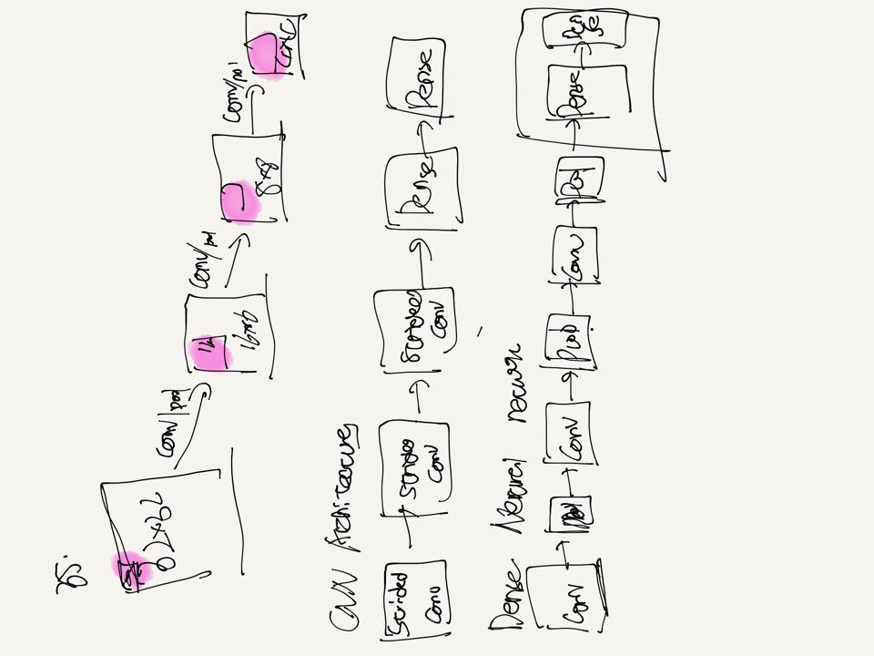
35. cnn architecture

CNN has two steps:

pooling

high level, pooling is downsampling

eg. output a smaller images from a bigger image

input 100x100 => pool size of 2 woule yield 50x50


Max pooling, average pooling 

Max pooling : 

why use pooling?

pattern finder에서 pattern이 found한 곳만 찾기 위해서 이다.


diferent pool sizes

stride : overlap이 가능하다.


pooling

conv-pool shrinks


losing information

Dowe lose information if we shrink the image ? Yes!

We lose spatial information : we don't care where the feature was found


hyperparameters: 

learning rate, hidden layers, hidden units per layer


pooling : stride


pixel


Dense Neural Network: 1xD layer


global max pooling


36. cnn code preparation(part1)

build the model

C1 x H x W x C2

nn.Conv2d(in_channels =1, out_channels = 32, kernel_size = 3, stride =2)

color images 3-d


color is not a spatial dimension

1-D convolution example: time series

3-D convolution example: video (height, width, time)

3-D convolution example: voxels(height, width, depth)
"pixel" = "Picture Element"

"Voxel" = "Volume Element"


conv2d -> conv2d -> conv2d -> flatten -> Dense -> Dense

conv2d = Image

Dense = Vector


ANN Review

model = nn.Sequential(

 nn.Linear(784128),

 nn.ReLU(),

 nn.Linear(12810)

)


class ANN(nn.Modeuls):

  def __init__(self):

    super(ANN, self).__init__()

    self.layer1= Linear(784128),

    self.layer2= ReLU()

    self.layer3 =Linear(128,1)

def forward(self, x):

    x = self.layer1(x)

    x = self.layer2(x)

    x = self.layer3(x)

    return x

model = ANN()


Linear model

variable = nn.Linear(D,1)

outputs = variable(inputs)


class CNN(nn.Module):


  def __init__(self):

    super(CNN, self).__init__()

    self.conv = nn.Sequential(

     nn.Conv2d(2, 32, kernel_size =3, stride=2)

     nn.Conv2d(32, 64, kernel_size =3, stride=2)

     nn.Conv2d(64, 128, kernel_size =3, stride=2)

    )

    self.dense = nn.Sequential(

      nn.Linear(?, 1024)

      nn.Linear(1024, K))

  def forward(self, x):

    out = self.conv(x)

    out = out.view(-1,?)

    out = self.dense(out)

    return out


CNN Sequentail version

model = nn.Sequential(

  nn.Conv2d(3, 32, kernel_size=3, stride =2)

  nn.Conv2d(32, 64, kernel_size=3, stride =2)

  nn.Conv2d(64, 128, kernel_size=3, stride =2)

  nn.Flatten()

  nn.Linear(?, 1024)

  nn.Linear(1024, K)

)


dropout Regularization:

L1 and L2 Regularization

dense layers

보통 dropout는 dense layer 사이에 사용한다.convolutions에 사용하지 않는다.

and sometimes RNNs


37. cnn code preparation(part2)

fill in the detaill

Convolutioanal Arithmetic

model = nn.Sequential(

  nn.Conv2d(3, 32, kernel_size=3, stride =2)

  nn.Conv2d(32, 64, kernel_size=3, stride =2)

  nn.Conv2d(64, 128, kernel_size=3, stride =2)

  nn.Flatten()

  nn.Linear(?, 1024)

  nn.Linear(1024, K)

)


keras 

32->16->8->4

"padding" argument


 중요한 점 

pytorch 특이한 점

why NxCxHxW and not NxHxWxC?

Conventions = whatever the programmer decided to do

Theano / Pytorch == channels first

OpenCV, Tensorflow, Matplotlib, pillow == channels last

OpenDV == BGR instead of RGB (try imread and then plot with Maplotlib)


38. cnn code preparation(part3)

1.load in the data

Fashion MNIST and CIFAR -10

2. BUILD THE MODEL ->convolutional 

3. TRAIN the model

4. evaluate the model

5. make predictions


"all machine learning interfaces are the same"


load in the data


data augmentation


Pytorch loading in the data

train_dataset = torchvision.datasets.FashionMNIST(

  root = '.',

  train = True

  transform = transforms.ToTensor(),

  download = True)


train_dataset = torchvision.datasets.CIFAR10(

  root = '.',

  train = True

  transform = transforms.ToTensor(),

  download = True)


train_loader = torch.utils.data.DataLoader(dataset = train_dataset, batch_size = batch_size, shuffle = True)


all data is the same

all machine learning interfaces are the same


Training loop

for i in rage(epochs):

  for inputs, targets in data_loader:

    ...


evaluating accuracy

for inputs, targets in data_loader:

  ...


39. cnn for fashion mnist

import torch
import torch.nn as nn
import torchvision
import torchvision.transforms as transforms
import numpy as np
import matplotlib.pyplot as plt
from datetime import datetime


train , test set 가져오기 

train_dataset = torchvision.datasets.FashionMNIST(
  root = '.',
  train = True, 
  transform = transforms.ToTensor(),
  download = True)
test_dataset = torchvision.datasets.FashionMNIST(
  root = '.',
  train = False, 
  transform = transforms.ToTensor(),
  download = True)


class 종류 확인하기

classes = len(set(train_dataset.targets.numpy()))
print("number of classes:", classes)

class CNN(nn.Module):
  def __init__(self, classes):
    super(CNN, self).__init__()

    self.conv_layers = nn.Sequential(
      nn.Conv2d(in_channels=1, out_channels = 32, kernel_size =3, stride=2),
      nn.ReLU(),
      nn.Conv2d(in_channels=32, out_channels = 64, kernel_size =3, stride=2),
      nn.ReLU(),
      nn.Conv2d(in_channels=64, out_channels = 128, kernel_size =3, stride=2),
      nn.ReLU()
    )
    self.dense_layers = nn.Sequential(
      nn.Dropout(0.2),
      nn.Linear(128*2*2, 512),
      nn.ReLU(),
      nn.Dropout(0.2),
      nn.Linear(512, classes)
    )

  def forward(self, x):
    out = self.conv_layers(x)
    out = out.view(out.size(0), -1)
    out = self.dense_layers(out)
    return out


model = CNN(classes)


다른 또 한가지 방법 tensorflow

'''
model = nn.Sequential(
  nn.Conv2d(in_channels=1, out_channels = 32, kernel_size =3, stride=2),
  nn.ReLU(),
  nn.Conv2d(in_channels=32, out_channels = 64, kernel_size =3, stride=2),
  nn.ReLU(),
  nn.Conv2d(in_channels=64, out_channels = 128, kernel_size =3, stride=2),
  nn.ReLU(),
  nn.Flatten(),
  nn.Dropout(0.2),
  nn.Linear(128*2*2, 512),
  nn.ReLU(),
  nn.Dropout(0.2),
  nn.Linear(512, classes) 
)
'''


model to gpu

device = torch.device("cuda:0" if torch.cuda.is_available() else 'cpu')
print(device)
model.to(device)


criterion = nn.CrossEntropyLoss()
optimizer = torch.optim.Adam(model.parameters())
batch_size = 128
train_loader = torch.utils.data.DataLoader(dataset = train_dataset, batch_size = batch_size, shuffle = True)
test_loader = torch.utils.data.DataLoader(dataset = test_dataset, batch_size = batch_size, shuffle = False)
def batch_gd(model, criterion, optimizer, X_train, y_train, epochs):
  train_losses = np.zeros(epochs)
  test_losses = np.zeros(epochs)

  for epoch in range(epochs):
    t0 = datetime.now()
    train_loss = []

    for inputs, targets in train_loader:
      inputs, targets = inputs.to(device), targets.to(device)
      optimizer.zero_grad()

      outputs = model(inputs)
      loss = criterion(outputs, targets)

      loss.backward()
      optimizer.step()

      train_loss.append(loss.item())

    train_loss = np.mean(train_loss)


    test_loss = []

    for inputs, targets in test_loader:
      inputs, targets = inputs.to(device), targets.to(device)
      outputs = model(inputs)
      loss = criterion(outputs, targets)
      test_loss.append(loss.item())
    test_loss = np.mean(test_loss)

    train_losses[epoch] = train_loss
    test_losses[epoch] = test_loss

    dt = datetime.now() - t0
    print(f'Epoch{epoch+1}/{epochs}, Train loss:{train_loss:.4f}, Test loss:{test_loss:.4f}')

  return train_losses, test_losses
train_losses, test_losses = batch_gd(model, criterion, optimizer, train_loader, test_loader, epochs=15)

정확도 구하기

n_correct = 0.
n_total = 0.
for inputs, targets in train_loader:
  inputs, targets = inputs.to(device), targets.to(device)
  outputs = model(inputs)
  _, predictions = torch.max(outputs, 1)
  n_correct += (predictions == targets).sum().item()
  n_total+= targets.shape[0]
train_acc = n_correct/ n_total
  
n_correct = 0.
n_total = 0.
for inputs, targets in test_loader:
  inputs, targets = inputs.to(device), targets.to(device)
  outputs = model(inputs)
  _, predictions = torch.max(outputs, 1)
  n_correct += (predictions == targets).sum().item()
  n_total+= targets.shape[0]
test_acc = n_correct/ n_total
print(f"Train acc: {train_acc:.4f} , Test acc:{test_acc:.4f}")
from sklearn.metrics import confusion_matrix
import numpy as np
import itertools
def plot_confusion_matrix(cm, classes, normalize = False, title =' Confusion matrix', cmap = plt.cm.Blues):
  if normalize:
    cm = cm.astype('float') / cm.sum(axis=1)[:, np.newaxis]
    print("Normalized confusion matrix")
  else:
    print("confusion_matrix: without Normalized")
  print(cm)
  plt.imshow(cm, interpolation='nearest', cmap=cmap)
  plt.title(title)
  plt.colorbar()
  tick_marks = np.arange(len(classes))
  plt.xticks(tick_marks, classes, rotation = 45)
  plt.yticks(tick_marks, classes)

  fmt ='.2f' if normalize else 'd'
  thresh = cm.max()/2
  for i, j in itertools.product(range(cm.shape[0]), range(cm.shape[1])):
    plt.text(j, i, format(cm[i,j], fmt), horizontalalignment="center" , color="white" if cm[i, j]> thresh else 'black')
  
  plt.tight_layout()
  plt.ylabel('True label')
  plt.xlabel('Predicted label')
  plt.show()
x_test = test_dataset.data.numpy()
y_test = test_dataset.targets.numpy()
p_test = np.array([])
for inputs, targets in test_loader:
  inputs = inputs.to(device)
  
  outputs = model(inputs)
  _, predictions = torch.max(outputs, 1)
  p_test = np.concatenate((p_test, predictions.cpu().numpy()))

cm = confusion_matrix(y_test, p_test)
plot_confusion_matrix(cm, list(range(10)))


p_test = p_test.astype(np.uint8)
misclassfied_idx = np.where(p_test != y_test)[0]
i = np.random.choice(misclassfied_idx)
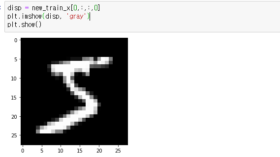
plt.imshow(x_test[i].reshape(28,28) , cmap = 'gray')
plt.title('True label: %s Predicted : %s' % (labels[y_test[i]], labels[p_test[i]]))

cnn better than ann


40. cnn for cifar-10

import torch
import torch.nn as nn
import torchvision
import torchvision.transforms as transforms
import numpy as np
import matplotlib.pyplot as plt
from datetime import datetime


cifar 10 dataset color imageset 

train_dataset = torchvision.datasets.CIFAR10(
  root = '.',
  train = True, 
  transform = transforms.ToTensor(),
  download = True)

test_dataset = torchvision.datasets.CIFAR10(
  root = '.',
  train = False, 
  transform = transforms.ToTensor(),
  download = True)

cifar 10 regular 

classes = len(set(train_dataset.targets))
print("number of classes: " , classes)

dataloader

batch_size = 128
train_loader = torch.utils.data.DataLoader(dataset = train_dataset, batch_size = batch_size, shuffle = True)
test_loader = torch.utils.data.DataLoader(dataset = test_dataset, batch_size = batch_size, shuffle = False)

cnn 정의 한다.

class CNN(nn.Module):
  def __init__(self, classes):
    super(CNN, self).__init__()
    self.conv1 = nn.Conv2d(in_channels=3, out_channels = 32, kernel_size =3, stride=2)
    self.conv2 = nn.Conv2d(in_channels=32, out_channels = 64, kernel_size =3, stride=2)
    self.conv3 = nn.Conv2d(in_channels=64, out_channels = 128, kernel_size =3, stride=2)
    self.fc1 = nn.Linear(128*3*3, 1024)
    self.fc2 = nn.Linear(1024, classes)

  def forward(self, x):
    x = F.relu(self.conv1(x))
    x = F.relu(self.conv2(x))
    x = F.relu(self.conv3(x))
    x = x.view(-1, 128*3*3)
    x = F.dropout(x, p =0.5)
    x = F.relu(self.fc1(x))
    x = F.dropout(x, p =0.2)
    x = self.fc2(x)
    return x
model = CNN(classes)


41. data augmentation

generators/ iterator

0.. 10: for i in range(10)

python 2 range(10)

python 2, use xrange(10)

python 3, print(range(10))

.....


for x in my_image_aumgmentation_generator():

  print(x)


def my_image_aumgmentation_generator():

  for x_batch, y_batch in zip(X_train, y_train):

    x_batch = gument(x_batch)

   yield x_batch, y_batch


Data augmentation with Torch Vision

transform = torchvision.transforms.Compose([

  torchvision.transforms.ColorJitter( 

    brightness=0.2, contrast = 0.2, saturation =0.2, hue =0.2),

    torchvision.transforms.RandomHorizontailFlip(p=0.5),

    torchvision.transforms.RandomRotation(degrees=15),

    transforms.ToTensor(),

  )

])


train_dataset = torchvision.datasets.CIFAR10(

  root = '.',

  train=True,

  transform = transform,

  download = True

)


dataloader은 그래도 한다. 이전과 같이 진행하면 된다. 


 Data Augmentation with your data

train_dataset = torchvision.datasets.yourdataset?(

  root = '.',

  train=True,

  transform = transforms.ToTensor(),

  download = True

)


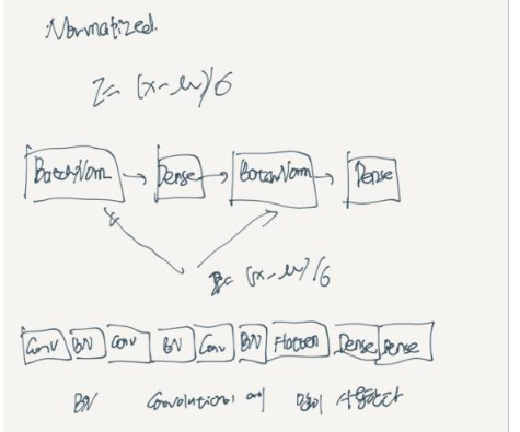
42. Batch Normalization

z = (x - μ) / σ 


for epoch in ragne(epochs):

  for x_batch, y_batch in data_loader:

    x<- w - learning_rate * grad(x_batch , y_batch)


Dense 사이에 한다.


Batch Norm as regularization

can help with overfitting

43. Improving CIFAR -10 Results


pytorch data augmentation

data augmentation

train_transform = torchvision.transforms.Compose([
  tranforms.RandomCrop(32, padding = 4),
  torchvision.transforms.RandomHorizontalFlip(p=0.5),
  torchvision.transforms.RandomAffine(0, translate=(0.1,0.1)),
  tranforms.ToTensor(),
])

train_dataset = torchvision.datasets.CIFAR10(
  root = '.',
  train = True, 
  transform = train_transform,
  download = True)

test_dataset = torchvision.datasets.CIFAR10(
  root = '.',
  train = False, 
  transform = train_transform,
  download = True)

모델 생성

maxpooling 

class CNN(nn.Module):
  def __init__(self, classes):
    super(CNN, self).__init__()
    self.conv1 = nn.Sequential(
        nn.Conv2d(3, 32, kernel_size= 3, padding =1 ),
        nn.ReLU(),
        nn.BatchNorm2d(32),
        nn.Conv2d(32, 32, kernel_size=3, padding=1),
        nn.ReLU(),
        nn.BatchNorm2d(32),
        nn.MaxPool2d(2),
    )
    self.conv2 = nn.Sequential(
        nn.Conv2d(32, 64, kernel_size= 3, padding =1 ),
        nn.ReLU(),
        nn.BatchNorm2d(64),
        nn.Conv2d(64, 64,kernel_size=3, padding=1),
        nn.ReLU(),
        nn.BatchNorm2d(64),
        nn.MaxPool2d(2),
    )
    self.conv3 = nn.Sequential(
        nn.Conv2d(64, 128, kernel_size= 3, padding =1 ),
        nn.ReLU(),
        nn.BatchNorm2d(128),
        nn.Conv2d(128, 128,kernel_size=3, padding=1),
        nn.ReLU(),
        nn.BatchNorm2d(128),
        nn.MaxPool2d(2),
    )
    self.fc1 = nn.Linear(128 * 4 * 4, 1024)
    self.fc2 = nn.Linear(1024, classes)
  def forward(self, output):
    output = self.conv1(output)
    output = self.conv2(output)
    output = self.conv3(output)
    output = output.view(output.size(0) , -1)
    output = F.dropout(output, p = 0.5)
    output = F.relu(self.fc1(output))
    output = F.dropout(output, p = 0.2)
    output = self.fc2(output)
    return output

vgg mach larger images 


from torchsummary import summary
summary(model, (3,32,32))
반응형
반응형

아래 내용은 Udemy에서 Pytorch: Deep Learning and Artificial Intelligence를 보고 정리한 내용이다.


22. Artificial Neural Networks Section introduction

CNNs

RNNs


Artificial Neural Networks: ANNs

neural networks


http://alexlenail.me/NN-SVG/index.html

activation functions:

These are what make neural networks 활성화 되는지 

Multiclass classification: 여러개 구분하는 것

Image data: images,. text, and sound


23. Forward Propagation

nerual networks -> predictions


E.g.: input is a face

one neuron 는 the presence of an 눈을 보고 

one neuron 는 the presence of an 코를 보고 

그들은 각각 다른 feature를 보고 있다.


input hidden output

layer

a chain of nerons

uniform structure


y =  wx+b

y = ax+b


sigmoid


앞의 neural network output을 구한다음 뒤어로 전달하면서 계싼한다.


regression

dense layer -> dense layer -> dense layer -> linear regression

classification

dense layer -> dense layer -> dense layer -> logistic regression


Hierachies

solve the compelicated problem


24. The Geometric Picture

geometric picture

feature engineering

linear regression

y hat = ax^2 + b

gradient descent


25. Activation Functions

sigmoid 0~1

 f(x) = 1 / 1 + exp(-a)

binary classification


standardization


tanh  -1~1 


vanishing gradient problem

변화가 거의 나지 않을 경우 


deaad end

default : Relu 

  doesn't have a "vaishing' gradient..

  the gradient in the left half is aleady vanished!


BRU activation

 higher accuracy


softplus


biological plausibility


26. Multiclass Classification

softmax function

softmax technically an activation function , but unlike the sigmoid/tahh, ReLU hidden activations는 아니다.

pytorch softmax function

nn.Sequential(

  nn.Linear(D,M),

  nn.ReLU(),

  nn.Linear(M, K),

  nn.Softmax()

)


crossEngropyLoss()


model = nn.Linear(D,K)

criterion = nn.CrossEntropyLoss()


activation function

task activation function
Regression None/Identity
binary classification sigmoid
multiclass classification softmax


The Model Type Doesn't matter


linear regression

dense


ann Regression 

dense + Dense


binary Logistic Regression

Dense+sigmoid


ANN Binary Classification

Dense+Dense+sigmoid


Multicalss Logistic Regression

Dense+ Softmax

ANN Multiclass Classification

Dense+Dense+ Softmax


same pattern applies to CNNs,RNNs - the type of task corresponds only to the final activation function


softmax is more general

multiclass classification

binary classification k = 2

27. How to Represent Images

이미지가 어떻게 데이터에 입력 되는지 확인 해야 한다.

height/width

matrix

column of the image


colors?

RGB  red/green/bue

black = 0

white  = 255


Images as input to neural networks

0 ... 255

feature vector


3dimensions: height,width , color


quantization:

color is light, measured by light intensity

fugured out that 8 bits(1byte)

2^3 => 0 ~ 255 

=> 500 x 500의 이미지는 얼마 만큼의 space를 찾이하는가 ?

500 x 500 x 3 x 8 = 6 million bits

jepg allows us to compress images


Hex Colors

each byte( 8 bits)


Grayscale Images : not have color 

2- D array (height, width)

black = 0 , white = 255

only be a white and black

plt.imshow() 

plt.imshow( , cmap ='gray') 


Images as input to neural networks

0...1  => 사이가 편하다.


Another exception 

VGG

images are centered around 0, but the range is still 256


Images as input to neural networks

N = #samples, D = #features

input X of shape NxD

A single image is HxWxC 

N x HxWxC 


Image to Feature Vector

reshape() or view()

NxD  array

28. Code Preparation (ANN)

1. load int the data

       MNIST dataset ->handwrite

2. build the model

3. train the model

4. evaluate the model

5. make the predictions


pytorch load MNIST

step1. load in the data -> pytorch library

grascale => 28x28 

train_dataset = torchvision.datasets.MNIST(

root = '.',

train = True, 

download = True)

x_train = train_dateset.data

y_train = train_dateset.targets

x_train.shape = N x 28 x 28

y_train.shape = N

n = 60,000


test_dataset = torchvision.datasets.MNIST(

root = '.',

train = False, 

download = True)

x_test = test_dataset.data

y_test = test_dataset.targets

x_test.shape = Ntest x 28 x 28

y_test.shape = Ntest

Ntest = 1,000


trainsforming the data

# reshape the input  -> small range

inputs = inputs.view(-1, 784)


step 2. model

model = nn.Sequential(

 nn.Linear(784, 128),

 nn.ReLU(),

 nn.Linear(128, 10)

)

10->  classification 결과 


step 3. trian the model

batch gradient Descent

for epoch in range(epochs):

  for x_batch, y_batch in batches(X,Y , batch_size = 128): => batch_size로 나누어서 학습 한다.

    train(x_batch, y_batch)


Batch Gradient Descent in pytTorch

train_loader = torch.utils.data.DataLoader(dataset = train_dataset, batch_siz e= batch_size, shuffle = True)


for epoch in range(epochs):

  for inputs, targets in train_loader:

    optimizer.zero_grad()


ramdom sample


step 4/5

n_correct = 0

n_total = 0

for inputs, targets in train_loader:

  output = model(inputs)


acc = n_correct/ n_total


_, predictions = torch.max(outputs, 1)


29. ANN for Image Classification

import torch
import torch.nn as nn
import torchvision
import torchvision.transforms as transforms
import numpy as np
import matplotlib.pyplot as plt
train_dataset = torchvision.datasets.MNIST(
  root = '.',
  train = True, 
  transform = transforms.ToTensor(),
  download = True)
train_dataset.data

train_dataset.data.max()

train_dataset.data.shape

train_dataset.targets


이미 다운로드 되여서 다운로드 하지는 않는다.

train_dataset = torchvision.datasets.MNIST(
  root = '.',
  train = True, 
  transform = transforms.ToTensor(),
  download = True)

model = nn.Sequential(
 nn.Linear(784, 128),
 nn.ReLU(),
 nn.Linear(128, 10)
)
# no need for final softmax!

gpu를 사용  여부 확인하면서 있을 경우 사용한다.

속도와 관련 있다. 

device = torch.device("cuda:0" if torch.cuda.is_available() else 'cpu')
print(device)
model.to(device)

loss and optimizer

ctriterion = nn.CrossEntropyLoss()
optimizer = torch.optim.Adam(model.parameters())
batch_size = 128
train_loader = torch.utils.data.DataLoader(dataset = train_dataset, batch_size = batch_size, shuffle = True)
test_loader = torch.utils.data.DataLoader(dataset = test_dataset, batch_size = batch_size, shuffle = False)


tmp_loader = torch.utils.data.DataLoader(dataset = train_dataset, batch_size = 1, shuffle = True)
tmp_loader

for x,y in tmp_loader:
    print(x)
    print(x.shape)
    print(y.shape)
    break

train_dataset.transform(train_dataset.data.numpy()).max()
epochs= 10

train_losses = np.zeros(epochs)
test_losses = np.zeros(epochs)

for epoch in range(epochs):
  train_loss = []
  for inputs, targets in train_loader:
    inputs, targets = inputs.to(device) , targets.to(device)

    inputs = inputs.view(-1, 784)
    optimizer.zero_grad()

    outputs = model(inputs)
    loss = ctriterion(outputs, targets)

    loss.backward()
    optimizer.step()

    train_loss.append(loss.item())
  
  train_loss = np.mean(train_loss)

  test_loss = []
  for inputs, targets in test_loader:
    inputs, targets = inputs.to(device) , targets.to(device)

    inputs = inputs.view(-1, 784)
    optimizer.zero_grad()

    outputs = model(inputs)
    loss = ctriterion(outputs, targets)

    test_loss.append(loss.item())
  
  test_loss = np.mean(test_loss)

  train_losses[epoch] = train_loss
  test_losses[epoch] = test_loss
  print(f'Epoch {epoch+1} / {epochs} , train loss : {train_loss:.4f} , Test loss: {test_loss:.4f}')


plt.plot(train_losses, label ='train loss')
plt.plot(test_losses, label = 'test loss')
plt.legend()
plt.show()

n_correct = 0.
n_total = 0.
for inputs, targets in train_loader:
  inputs, targets = inputs.to(device), targets.to(device)
  inputs = inputs.view(-1, 784)
  outputs = model(inputs)
  _, predictions = torch.max(outputs, 1)
  n_correct += (predictions == targets).sum().item()
  n_total+= targets.shape[0]
train_acc = n_correct/ n_total
  
n_correct = 0.
n_total = 0.
for inputs, targets in test_loader:
  inputs, targets = inputs.to(device), targets.to(device)
  inputs = inputs.view(-1, 784)
  outputs = model(inputs)
  _, predictions = torch.max(outputs, 1)
  n_correct += (predictions == targets).sum().item()
  n_total+= targets.shape[0]
test_acc = n_correct/ n_total
print(f"Train acc: {train_acc:.4f} , Test acc:{test_acc:.4f}")
from sklearn.metrics import confusion_matrix
import numpy as np
import itertools
def plot_confusion_matrix(cm, classes, normalize = False, title =' Confusion matrix', cmap = plt.cm.Blues):
  if normalize:
    cm = cm.astype('float') / cm.sum(axis=1)[:, np.newaxis]
    print("Normalized confusion matrix")
  else:
    print("confusion_matrix: without Normalized")
  print(cm)
  plt.imshow(cm, interpolation='nearest', cmap=cmap)
  plt.title(title)
  plt.colorbar()
  tick_marks = np.arange(len(classes))
  plt.xticks(tick_marks, classes, rotation = 45)
  plt.yticks(tick_marks, classes)

  fmt ='.2f' if normalize else 'd'
  thresh = cm.max()/2
  for i, j in itertools.product(range(cm.shape[0]), range(cm.shape[1])):
    plt.text(j, i, format(cm[i,j], fmt), horizontalalignment="center" , color="white" if cm[i, j]> thresh else 'black')
  
  plt.tight_layout()
  plt.ylabel('True label')
  plt.xlabel('Predicted label')
  plt.show()


x_test = test_dataset.data.numpy()
y_test = test_dataset.targets.numpy()
p_test = np.array([])
for inputs, targets in test_loader:
  inputs = inputs.to(device)

  inputs = inputs.view(-1, 784)
  
  outputs = model(inputs)
  _, predictions = torch.max(outputs, 1)
  p_test = np.concatenate((p_test, predictions.cpu().numpy()))

cm = confusion_matrix(y_test, p_test)
plot_confusion_matrix(cm, list(range(10)))


결과가 안같은 것 보여주기 

misclassified_idx = np.where(p_test != y_test)[0]
i = np.random.choice(misclassified_idx)
plt.imshow(x_test[i], cmap ='gray')
plt.title("True label: %s Predicted: %s" % (y_test[i], int(p_test[i])))


30. ANN for Regression

pytorch regression

import torch
import torch.nn as nn
import numpy as np
import matplotlib.pyplot as plt
from mpl_toolkits.mplot3d import Axes3D
N = 1000
X = np.random.random((N,2)) * 6 -3
y = np.cos(2 * X[:,0]) + np.cos(3*X[:,1])
fig = plt.figure()
ax = fig.add_subplot(111, projection='3d')
ax.scatter(X[:,0] , X[:,1] , y)

notebook과 다른점은 plt.show()할 필요 없다.


모델 생성하기

#build the model

model = nn.Sequential(
    nn.Linear(2, 128),
    nn.ReLU(),
    nn.Linear(128, 1)
)
criterion = nn.MSELoss()
optimizer = torch.optim.Adam(model.parameters(), lr = 0.01)
def full_gd(model, criterion, optimizer, X_train, y_train, epochs= 1000):
  train_losses = np.zeros(epochs)

  for epoch in range(epochs):
    optimizer.zero_grad()

    outputs = model(X_train)
    loss = criterion(outputs, y_train)

    loss.backward()
    optimizer.step()

    train_losses[epoch] = loss.item()

    if(epoch+1) % 50 == 0:
      print(f'Epoch {epoch+1}/{epochs}, Train loss:{loss.item():.4f} ')

  return train_losses

X_train = torch.from_numpy(X.astype(np.float32))
y_train = torch.from_numpy(y.astype(np.float32).reshape(-1,1))
train_lossses = full_gd(model, criterion, optimizer, X_train, y_train)
plt.plot(train_losses)

fig = plt.figure()
ax = fig.add_subplot(111, projection = "3d")
ax.scatter(X[:,0] , X[:,1] , y)

with torch.no_grad():
  line = np.linspace(-3, 3, 50)
  XX, yy = np.meshgrid(line, line)
  Xgrid = np.vstack((XX.flatten(), yy.flatten())).T
  Xgrid_torch = torch.from_numpy(Xgrid.astype(np.float32))
  yhat = model(Xgrid_torch).numpy().flatten()
  ax.plot_trisurf(Xgrid[:, 0] , Xgrid[:, 1] , yhat, linewidth = 0.2 , antialiased = True)
  plt.show()


아래 그림은 더 크게 만들어준다.

fig = plt.figure()
ax = fig.add_subplot(111, projection = "3d")
ax.scatter(X[:,0] , X[:,1] , y)

with torch.no_grad():
  line = np.linspace(-5, 5, 50)
  XX, yy = np.meshgrid(line, line)
  Xgrid = np.vstack((XX.flatten(), yy.flatten())).T
  Xgrid_torch = torch.from_numpy(Xgrid.astype(np.float32))
  yhat = model(Xgrid_torch).numpy().flatten()
  ax.plot_trisurf(Xgrid[:, 0] , Xgrid[:, 1] , yhat, linewidth = 0.2 , antialiased = True)
  plt.show()

반응형

+ Recent posts