논문 : Rethinking the Inception Architecture for Computer Vision 2016

suitably factorized convolutions 와 aggressive regularization

scaling up convolution networks in efficient ways

factorizing convolution

dimension reduction

batch-normalized auxiliary classifiers and label-smoothing

Abstract

Convolutional networks는 다양한 분야에서 state-of-the-art성능을 가진  computer vision 솔루션이다. 2014부터  deep convolutional networks 은 주류화되기 시작하여 , 다양한  benchmarks에서 상당한 이득을 얻었다 . model size 와 computational cost 증가하면 most tasks에 대한 즉각적인 성능 품질 향상 으로 이루어지는 경향이 있지만 (레이블링된 데이터가 학습을 위해 충분히 제공되는 한) , computational efficiency 와 low parameter count 는 여전히 mobile vision  및 big-data scenarios 와 같은 다양한 사용 사례에 대한 요소를 가능하게 한다. 여기서 우리는 suitably factorized convolutions 와 aggressive regularization 를 통해 추가된 계산을 최대한 효율적으로 활용하는 것을 목표로 네트워크를 확장하는 방법을 탐색하고 있다. 우리는 ILSVRC 2012 classification challenge validation set에 테스트 하여  state of the art 기법에 대해 상당한 이득을 입증한다. inference 당   computational cost이 less than 25 million parameters 5 billion multiply-adds인 네트워크를 가지고 테스트 한 결과는 다음과 같다. 

single frame evaluation  21.2% top-1 and 5.6% top-5 error  

4 models와 multi-crop evaluation로 구성된 앙상블을 통해 3.5% top-5 error and 17.3% top-1 error 를 보고한다. 

1. Introduction

2012년 “AlexNet” 성공한 이후 다양안 큰 컴퓨터 비전 작업이 적응되였다. 예를 들면 : object-detection [5], segmentation [12], human pose estimation [22], video classification [8], object tracking [23], and superresolution [3].

이것을 성공으로 인하여  convolutional neural networks를 찾는데 집중하였다.  2014년 이후로는  ,더  깊고 넓어진 네network architectures  를 활용하여 network architectures 의 성능이 크게 향상됬다 . VGGNet [18] and GoogLeNet [20] 2014 ILSVRC [16] classification challenge 에서 비슷하게 높은 성능을 가졌다. 한가지  흥미로운 관찰은 분류 성능을 얻기 위해서 다양한 응용 분야에서 상당한 품질 향상으로 이동하는 경향이 있다는 것이다. => application domains . 이는 deep convolutional architecture 의 구조적 개선이 high quality의 학습된 visual features에 점점 더 의존하는 대부분의 다른 컴퓨터 비전 작업에 대한 성능 향상에 활용될 수 있음을 의미한다.  또한, network quality 의 품질의 개선은 AlexNet  기능이 검출에서의 제안 생성과 같이 hand engineered, crafted solutions ( e.g. proposal generation in detection[4])과 경쟁할 수 없는 경우에 컨볼루션 네트워크를 위한 새로운 애플리케이션 도메인으로 이어졌다. 

VGGNet[18]은 architectural simplicity이라는 매력적인  특징을 가지고 있지만, 네트워크를 평가하는데 많은 계산이 필요하다. 반면에  , Inception아키텍츠의 GoogLeNet [20]의 Inception architecture는 메모리와 계산 예산에 대한 엄격한 제약 속에서도 잘 작동하도록 설계되었다.예를 들면 :

GoogleNet 5 million parameters 변수만을 사용했는데 

AlexNet은 약 60 million parameters 

VGGNet은 AlexNet의 3배이고 

GoogleNet은 AlexNet 보다 12배 적게 

Inception 의 computational cost은 또한 VGGNet나 혹은 보다 좋은 성능의 후속 네트워크들보다 훨씬 적다. 이로 인해 모바일과 같이 memory나 computational capacity가 제한된 환경에서  합리적인 비용으로 처리해야 하는 big-data scenarios[17], [13], 를 다루는 경우에 inception network를 활용할 수 있다. 물론, memory use [2], [15] 에 특화된 솔루션을 적용하거나 , computational tricks [10]으로  통해 특정 작업의 실행을 최적화함으로써 이러한 문제의 일부를 완화할 수 있다. 그러나 이러한 방법은 복잡성을 가중시키고 더욱이 이러한 방법들은 Inception architecture를 최적화 하는  데도 적용되어 효율성 격차를 다시 확대할 것이다. 

그럼에도 불구하고, Inception architecture의 복잡성은 network을 더욱 어렵게 만든다. architecture 가 순수하게 확장되는 경우, 계산 이득의 많은 부분이 즉시 손실될 수 있다. 또한,  [20] Google Net architecture은 다양한 design decisions 으로 이어지는 contributing factors에 대해 명확하게 설명하지 않았다. 이 것 때문에  효율성을 유지하면서 새로운 use-cases 적응하기가 훨씬 어려워진다. 예들 들어 일부 Inception-style model의 용량을 증가시킬 필요가 있다고 판단되는 경우, 모든 filter bank 크기의 수를 두 배로 늘리는 간단한 변환은 계산 비용과 매개변수 수 모두에서 4배 증가를 초래할 것이다. (filter back 2배 늘어나면 계산 비용과 매개변수 수  4배 ). 이는 특히 관련 이득이 크지 않은 경우, 많은 실제 시나리오에서 금지적이거나 비합리적인 (prohibitive or unreasonable)것으로 판명될 수 있다. => 불합리 본 논문에서는 convolution networks를 효율적으로 장하는 데 유용한 것으로 입증된 몇 가지 일반적인 원칙과 최적화 아이디어를 설명하는 것으로 시작한다. 우리의 원칙은  Inception-type networks에 국한하지 않지만, Inception style building blocks의 일반적인 구조는 그러한 제약 조건을 자연스럽게 통합할 수 있을 만큼 충분히 유연하기 때문에 그러한 맥락에서 관찰하기가 더 쉽다. 이는 인근 구성 요소에 대한 구조 변경의 영향을 완화할 수 있는 Inception module의 dimensional reduction 및 parallel structures를 관대하게 사용함으로써 가능하다. 그러나 모델의 높은 품질을 유지하기 위해서는 몇 가지 지침 원칙이 지켜져야 하기 때문에 그렇게 하는 데 신중할 필요가 있다.

2. General Design Principles

여기서 우리는 convolutional networks를 사용하여 다양한 architectural  선택 을 가진 대규모 실험 기반으로 하는 몇가지 설계 원리를  소계할 것이다. 이 시점에서는 , 아래 원칙들의 효용성은 추측적이며,  정확성과 유효성의 영역을 평가하기 위해 추가적인 실험 증거가 필요할 것이다.  그럼에도 불구하고, 이러한 원칙들로부터의 중대한 편차는 네트워크의 품질 저하를 초래하는 경향이 있으며, 그러한 편차가 감지된 상황을 수정하는 것은 일반적으로 architectures 개선을 초래하였다.

1. 특히 초기에 병목현상을 피하십시오. Feed-forward networks 는  input layer(s)에서 classifier or regressor간의  acyclic graph 표시 할 수 있다. 이는 명확하게 정보 흐름의 방향을 정의한다. inputs from the outputs을 구분하는 컷의 경우 컷을 통과하는 정보의 양에 액세스할 수있다. 극단적인 압축으로 인한 병목현상을 피해야 한다. 일반적으로 representation size는 used for the task at hand final representation 에 도달하기 전에 입력에서 출력으로 서서히 감소해야 한다. 이론적으로, 정보 내용은 상관 구조와 같은 중요한 요소를 무시하기 때문에 dimensionality of the representation 으로만 평가될 수 없다.

2. Higher dimensional representations 은 네트워크에서 local로 처리하기 더 쉽다. convolutional network 에서

per tile activations 을 늘리면  더 많은 disentangled features를 사용할 수 있다. 결과적으로 으로는 네트워크 학습이 더 빨리 될 것이다. 

3. Spatial aggregation는 표현력의 힘은 손실 없이 lower dimensional  임베딩을 통해 수행 할 수 있다. 예를 들어 , spread out (e.g. 3 × 3) convolution 을 수행하기 전에 ,  심각한 부작용없이  input representation의 dimension reduce 이 가능하므로 , spatial aggregation을 할 수 있다. 우리는 그 이유가 인접한 단위 결과 간의 강한 상관관계과 spatial aggregation context에서 출력을 사용하는 경우 dimension reduction 동안 정보의 손실을 훨씬 줄이기 때문이라고 가정한다. 이러한 신호가 쉽게 압축될 수 있어야 한다는 점을 고려하면, 차원 축소는 더 빠른 학습을 촉진한다.

4. network의 width and depth의 Balance 를 유지한다. per stage 별 filters 수와 network의 depth 의 균형을 유지함으로써 네트워크의 Optimal performance에 도달할 수 있다. network의 width and depth를 늘리면 더 높은 품질의 네트워크에 기여할 수 있다. 그러나 둘 다 병렬로 증가하면 일정한 양의 계산에 대한 최적의 개선에 도달할 수 있다. 따라서 computational budget은 network의 width and depth 사이에 균형 잡힌 방식으로 배분되어야 한다.

이러한 원칙이 타당할 수 있지만, 즉시 네트워크의 품질을 개선하기 위해 사용하는 것은 간단하지 않다. 애매한 상황에서만 현명하게 활용하자는 의미이다. 

3. Factorizing Convolutions with Large Filter Size

GoogLeNet network [20]의 원래 이득의 대부분은 차원축소를 매우 풍부하게 사용함으로써 발생한 것이다. 이것은  계산적으로의 factorizing convolutions 하는 특별한 경우로 볼수 있다. 예를 들어 1 × 1 convolutional layer 의 경우를 1x1 conv layer 다음에 3x3 conv layer가 오는 경우를 고려해보자 . vision network에서  near-by activations 의 출력은 상관관계가 높다는 것으로 예상된다.  따라서 우리는 그들의 집계전에 활성화를 줄일 수 있으며, 이는  유사한 지역 표현을 가지는 것으로 볼 수 있다. 

여기서는 특히 solution의 computational efficiency을 높이기 위해, 다양한 설정에서 convolutions 을 factorizing 하는 방법을 살펴본다. Inception networks 는 fully convolutional이기 때문에, 각 weight는 활성화당 하나의 곱셈에 해당한다. 따라서 computational cost 의 감소는 parameters의 number 를 감소한다. 이것은 적절한 factorization로 인해 더 많은 disentangled parameters 를 가질수 있고  따라서 더 빠른 훈련으로 끝날 수 있다는 것을 의미한다.  또한 computational and memory savings을 사용하여 network 의 filter-bank sizes를 늘리는 동시에 single computer에서 각 모델 복제본을 학습할 수 있는 능력을 유지할 수 있다. 

3.1. Factorization into smaller convolutions

더 큰 spatial filters (e.g. 5 × 5 or 7 × 7) 을 사용한  Convolutions 은 computation측면에서 disproportionally expensive경향이 있다. 예를 들어 , m개의 필터가 있는 그리드 위에 n개의 필터가 있는 5 × 5 convolution 은 동일한 filter 수가 3 × 3 convolution 에 비해 비용이 25/9 = 2.78배 더 비싸다.  ((5 × 5)/ (3 x 3) = 25 / 9) 물론 5 × 5 filter 는 earlier layers에서 멀리 떨어진 장치의 활성화 사이의 신호 간 의존성을 포착할 수 있으므로 필터의 geometric size를 줄이는 것은 표현력의 큰 비용을 지불하게 된다. 하지만 , 우리는 여기서 5 × 5 convolution는 input size and output depth가 동일한 parameters 를 적게 가진 multi-layer network로 대체될 수 있는지 물어볼 수 있느냐.  5 × 5 convolution의 computation graph를 확대하면, 각 출력은 입력 위로 5 × 5 tiles  위로  sliding 는 작은 fully-connected network처럼 보인다. vision network를 구축하기 때문에, translation invariance 을 다시 활용하고 fully connected 된 구성요소를 two layer convolutional architecture로 대체하는 것이 자연스러운 것으로 보인다. 

첫번째 레이어 : 3 × 3 convolution

두번째 레이어 : first layer 3 × 3 output grid 위에 fully connected layer  (see Figure 1). 

input activation grid위로 이 작은 network 를 Sliding 하는 것은 5 × 5 convolution을 2개의 3 × 3 convolution (compare Figure 4 with 5) 대체하는 것으로 요약된다 .

이 설정은 adjacent tiles에 weights 를 공유하여 parameter수를 명확하게 줄인다. 예상되는 computational cost savings 을 분석하기 위해 , 우리는 일반적인 상황에 적용되는 몇 가지 단순화된 가정을 할 것이다.  우리는 n = αm, 즉 일정한 알파 인자에 의해  활성화/단위의 수를 변경하고자 한다고 가정할 수 있다. 5 × 5 layer

에 대한 두 개의 레이어 교체가 있기 때문에, 두 단계 모두에서 필터 수를 √ α 만큼 증가시키는 두 단계로 이 확장에 도달하는 것이 타당해 보인다. (2-layer의 경우, 각 단계에서 filter 수를 √α만큼 증가시키는 방법을 취할 수 있다.) 만약 추정치를 단순화하기 위해α = 1 (no expansion), neighboring grid tiles사이의 computation 을 재사용하지 않고 network 를 단순히 slide 한다면, computational cost가 증가시킬 것이다. 이 network 를 sliding 하는 것은 adjacent tiles사이의 activations 를 재사용하는 two 3×3 convolutional layers로 나타낼 수 있다. 이러한 방식으로, 우리는 순 (9+9)/25 × 계산의 감소로 끝나게 되고, 이 인수 분해에 의해 28%의 상대적 이득을 얻는다. 각 parameter 가 각 unit의 activation  계산에 정확히 한 번 사용되므로 파라미터 카운트에 대해 정확히 동일한 저장이 유지된다. 그러나 이 설정에서는 다음과 같은 두 가지 일반적인 문제가 발생한다. 

1. replacement 으로 부터 expressiveness이 손실되는가 ?

2. 우리의 주요 목표가 계산의 linear part을 factorize 하는 것이라면, first layer에서 linear activations를 유지해야 하는가 ?

우리는 여러가지 control experiments(for example see figure 2)을 수행했으며 linear activation 를 사용하는 것은 , factorization의 모든 단계에서 rectified linear units를 사용하는 것보다 좋지 않았다.

저자들은 이러한 이득들이 특히 output activations를 batch-normalize [7]하는 network가 학습할 수 있는 향상된 space of variations 덕분이다고 한다. dimension reduction components에 linear activations를 사용할때도 비슷한 효과를 볼 수 있다.

3.2. Spatial Factorization into Asymmetric Convolutions

위의 결과는 큰 3 × 3 필터는 항상  3 × 3 convolutional layers의  sequence 로 축소될수 있기 때문에 일반적으로 유용하지 않을 수 있음을 시사한다.  여전히 우리는 예를 들어 2×2 convolutions과 같이 작은 단위로 인수분해해야 하는지에 대한 질문을 할 수 있다. 하지만 asymmetric convolutions, e.g. n × 1을 사용하면 2 × 2 보다 훨씬 더 잘 할 수 있다. 예들 들어 , 3 × 1 convolution 에 이어 1 × 3 convolution을 사용하는 것은 3 × 3 convolution (see figure 3)에 있는 것과 동일한 receptive fieldㄹㄹ 가진  two layer network 를 sliding하는 것과 같다. 그에 비해, 3 × 3 convolution 을 2개의 2 × 2 convolution으로 인수분해하는 것은 계산의 11% 절약을 나타낸다. 

이론적으로 , 우리는 더 나아가서 n × n convolution을 1 × n convolution이어서 n × 1 convolution을 대체할 수 있으며 계산 비용 절감은 n이 커질수록 극적으로 증가한다고 주장할 수 있다. (see figure 6). 실제로 , 우리는 이 factorization 를 사용하는 것이 

early layers에서는 잘 작동하지 않지만 medium grid-sizes(m×m 피처 맵에서는 m이 12~20 범위)에서는 매우 좋은 결과를 제공한다는 것을 발견하였다. 그 수준에서 1 × 7 convolutions에 이어 7 × 1 convolutions결과를 얻을 수 있다. 

4. Utility of Auxiliary Classifiers

[20] very deep networks 의 개념을 수렴하여 개선하는 auxiliary classifiers 의 개념을 도입했다. 원래의 동기는 유용한 gradients로 the lower layers로 밀어 즉시 유용하게 만들고 very deep networks에서 vanishing gradient problem를 해결함으로써 학습 중 수렴을 개선하는 것이었다.  또한 Lee et al[11]는 auxiliary classifiers보다 안정적인 학습과 더 나은 수렴을 촉진한다고 주장했다. 흥미롭게도, 우리는 auxiliary classifiers가 훈련의 초기에는 수렴을 개선하지 않았다는 것을 발견했다. side head가 있는 newtork와 없는 network의 훈련 진행은 두 모델이 높은 정확도에 도달하기 전에 사실상 같아 보인다. 훈련이 끝날 무렵, auxiliary branches 가 있는 network는 어떠한 것도 없이 network의 정확도를 추월하기 시작한다. 

플래토ː, plateau:무엇을 연습할 때, 처음에는 진보가 빠르나, 어느 단계에 이르면 진보가 멈추고 그 후 다시 연습을 계속하면 재차 진보하기 시작하는 상태. 고원 현상(高原現像).

또한 [20] network의 서로 다른 단계에서 두가지 side-heads를 사용했다. lower auxiliary branch의 제거는 network의 최종 품질에 악영향을 미치지 않았다. 이전 단락의 이전 관측과 함께, 이는 이러한 branches 가 low-level features 의 진화에 도움이 된다는 [20]의 원래 가설이 잘못되었을 가능성이 높다는 것을 의미한다. 대신에 , 우리는 auxiliary classifiers가 regularizer의 역할을 주장한다. 이것은 side branch가 batch-normalized [7] 되거나 dropout layer이 있는 경우 network의 main classifier가 더 잘 수행된다는 사실에 의해 뒷받침된다.  이것은 또한 batch normalization가 regularizer로서 작용한다는 대한 약한 근거를 제공한다. 

=>batch normalization acts as a regularizer

5. Efficient Grid Size Reduction

전통적으로 , convolutional networks 는 일부 pooling operation을 사용하여 feature maps의 grid size를 줄였다. representational bottleneck을 피하기 위해 maximum or average pooling전에 network filters의 activation dimension을 확장한다. 예를 들어, k filters로 d×d grid를 시작할때 , 2k filters로  (d/2) ×(d/2) grid 에 도착하면, 먼저 2k filters로 stride-1 convolution 을 계산한 다음 추가 pooling step를 적용해야 한다. 이는 전체 computational cost 이 2d^2k^2 연산을 사용하는 더 큰 grid의 expensive convolution에 의해 좌우된다는 것을 의미한다.  한가지 가능성은 convolution 을 사용한 pooling으로 전환하여   2*( d/2)^2*k^2로 계산 비용을 1/4로 절감하는 것이다. 그러나 , 이것은 표현의 전체 차원성이 (d/2)^2*k로 떨어져 representation 이 떨어지는 network를 만들면서 representational bottlenecks현상을 일어킨다. (see Figure 9).  그렇게 하는 대신, 우리는 representational bottleneck현상을 제거하는 계산 비용를 훨씬 더 절감하는 또 다른 변형을 제안했다. (see Figure 10) . 우리는 two parallel stride 2 blocks을 사용할 수 있어 P와 C. 

P: pooling layer (평균 또는 최대 pooling) activation

C: 둘다 그림 10과 같이 연결된 filter banks stride 2이다. 

6. Inception-v2

여기서 우리는 위에서 dots을 연결하고  ILSVRC 2012 classification benchmark에서 성능이 향상된 새로운 architecture 를 제안한다. 우리 network의 layour은 table 1에 나와 있다. section 3.1에서 설명한 것과 동일한 아이디어에 기초하여 7 × 7 convolution 을 3 × 3 convolutions으로 인수분해했다. network의 Inception 에서 , 우리는 각각  288 filters가 있는  35×35에 3개의 전통적인 Inception 모델을 가지고 있다. section 5에서 설명한 grid reduction techniqu을 사용하여 768개의 filter가 17 × 17 grid 로 축소된다. 이것은 figure 5에서 묘사된 것 과 같이 인수 분해된 inception modules 의 사례가 뒤따른다. 이것은  figure 10에 묘사된 grid reduction technique을 통해 8 × 8 × 1280 grid로 축소된다. 가장 coarsest 8 × 8 level에서, 우리는  figure 6에서 묘사된 것 처럼 각 tile에 2048인 두개의 Inception modules을 가지고 있다. Inception modules내부의 filter bank size를 포함함 network의 자세한 구조는 모델에 제시된 supplementary material에 제시되어 있다. 이 submission 의 tar 파일에 있는 model.txt이다. 그러나 Section 2의 원칙을 준수하는 한 network의 품질이 변화에 대해 상대적으로 안정적이라는 것을 관찰했다. network 깊이는 42 layers이지만, 계산 비용은 GoogLeNet보다 약 2.5배 더 높을 뿐이고 여전히 VGGNet보다 훨씬 효율적이다.

7. Model Regularization via Label Smoothing

여기서는 학습 중 label-dropout 의 한계 효과를 추정하여 classifier 계층을 정규화하는 메커니즘을 제안한다. 각 학습 데이터 x에 대해, 우리는 모델은 각 레이블

k ∈ {1 . . . K}: p(k|x) = p(k|x) = exp(z_k)/ \sum_{i=1}^kexp(z_i)

여기서 z_i는 logits 또는 unnormalized logprobabilities이다. 이 학습 예제의 레이블 q(k|x) 에 대한 ground-truth distribution 를  \sum_{k} q(k|x)=1 이 되도록 정규화한다 . 간략하게 하기 위해, 예제 x에서 p와 q의 의존성을 생략하라 . 우리는 예에 대한 손실을 교차 엔트로피 l = -\sum_{k=1}^Klog(p(k))q(k)로 정의한다.  이것을 최소화하는 것은 라벨이 ground-truth distribution q(k)에 따라 선택되는 라벨의 예상 log-likelihood of a label을 최대화하는 것과 같다. Cross-entropy loss는 logits z_k와 관련하여 구별할 수 있으므로 deep models의 gradient 학습에 사용될 수 있다. gradient 는 다소 단순한 형태를 가지고 있다.

\partial l / \partial z_k = p(k)-q(k) 

이며, -1과 1 사이의 경계이다. 

그래서 , k != y q(y) = 1 and q(k) = 0 이 되는 single ground-truth label y의 경우를 생각해 보십시오 . 이 경우 cross entropy를 최소화하는 것은 correct label the log-likelihood를 최대화 하는 것과 같다. label y이 있는 특정 예제 x의 경우 log-likelihood는 q(k) = δ k,y 에 대해 최대화 되며 여기서 δ k,y is Dirac delta이며, k=y일 때 1이고, 그렇지 않은 경우에는 0이다. 유한한 z_k에 대해 maximum 을 달성할수는 없지만, zy≫zk,∀k≠y의 경우에는 즉 ground-truth label에 해당하는 logit이 다른 logits 보다 훨씬 큰 경우에 접근한다. 그러나 이것은 두 가지 문제를 일으킬 수 있다.

1. over-fitting이 발생할 수 있다. model 이 각 학습 예제에 대해 ground-truth label의 모든 확률을 할당하도록 학습한다면, 일반화 성능을 조장할 수 없다.

2. largest logit 과 다른 all others to become large사이의 크기가 커지도록 장려하고 이는 bounded gradient ∂ℓ/∂zk 와 함께 사용하게 되면  모델의 적응 능력을 감소시킨다. 직관적으로 모형이 예측에 대해 너무 확신하기 때문에 이러한 현상이 발생한다.

우리는 모델이 덜 신뢰하도록 장려하기 위한 메커니즘을 제안한다.  training labels의 log-likelihood을 최대화하는 것이 목적인 경우에는 이 방법이 바람직하지 않을 수 있지만 모형을 정규화하고 적응성을 높인다. 방법은 매우 간단하다. training example x에 독립인 label distribution u(k)와 smoothing parameter인 ϵ을 고려한다. ground-truth label y일 때, label distribution q(k|x) = δ k,y 를 다음과 같이 바꿀 수 있다. 

q′(k∣x)=(1−ϵ)δk,y + ϵu(k)

original ground-truth distribution q(k|x) 와 the fixed distribution u(k) 에  1 − ϵ and ϵ 에 각각 weight 로 곱해진 혼합식이다. 

이것은 다음과 같이 얻은 레이블 k의 분포로 볼 수 있다: 

1. ground-truth label k = y를 설정한다. 

2. 그런 다음 확률이 ϵ, k를 distribution u(k)에서 추출한 표본으로 바뀐다. 

labels 에 대한 prior distribution를 u(k)로 용할 것을 제안한다. 실험에서 , uniform distribution u(k) = 1/K를 사용한다. q′(k)=(1−ϵ)δk,y+ϵKq′(k)=(1−ϵ)δk,y+ϵK.

우리는 ground-truth label distribution의 이러한 변화를 label-smoothing regularization, or LSR이라고 부른다. 

LSR 은 largest logit 이 다른 logit보다 훨씬 더 커지는 것을 방지하는 목적할 수 있다는 점에 유의 하십시오. 실제로, 만약 이것이 일어난다면, 다른 모든 q(k)는 0에 접근하는 반면, 단일 q(k)는 1에 접근할 것이다. 실제로 LSR이 적용되면, q′(k)는 큰 cross-entropy 값을 가지게 될 것이고 q′(k)가 δk,y와는 달리  positive lower bound가 있기 때무니다. 

LSR의 또 다른 해석은 cross entropy를 고려함으로써 얻을 수 있다. 

H(q′,p)=−∑Kk=1logp(k)q′(k)=(1−ϵ)H(q,p)+ϵH(u,p)

따라서 LSR은  single cross-entropy loss H(q,p) 를 그러한 losses H(q,p) and H(u,p)의 쌍으로 대체하는 것과 같다.  두번재 loss인 H(u,p)는 , prior u로 부터 얻어지는 predicted label distribution p의 deviation 에 대해 계산되며 , 첫번째 loss에 비해 상대적으로 ϵ/(1−ϵ)만큼 가중된다. H(u,p) = D KL (ukp) + H(u)및  H(u)가 고정되었기 때문에 KL divergence에 의해 동등하게 포착될 수 있다. u 가 uniform distribution일 때 , H(u,p)는 predicted distribution p 는 uniform 하지 않는 지에 대한 측도이다. negative entropy −H(p)에 대해서 측정할 수 있지만 동일한 값은 아니다 .K = 1000 classes를 사용한  ImageNet experiments에서 u(k) = 1/1000 and ϵ = 0.1을 사용했다. ILSVRC 2012의 경우, top-1 error and the top-5 error (cf. Table 3) 모두에 대해  0.2%의 절대적인 개선을 발견했다. 

8. Training Methodology

TensorFlow [1] distributed machine learning system에서 50 replicas running 이 각각 NVidia Kepler GPU 상에서 stochastic gradient로 학습됐다.  

batch size 32 for 100 epochs .

초반 실험에서는 decay가 0.9인 momentum[19]을 사용했었으며,

best model은 decay가 0.9인 RMSProp[21] 과, ϵ=1.0 ϵ=1.0을 사용할 때 얻었다.

Learning rate는 0.045에서 시작하여, 두 번의 epoch마다 0.94를 곱했다. 또한, threshold가 2.0인 gradient clipping [14] 이 안정적인 학습에 도움된다는 것을 발견했다.

모델의 평가는, 시간이 지남에 따라 계산 된 parameter의 running average을 사용하여 수행한다. 

9. Performance on Lower Resolution Input

vision networks의 일반적인  예를 들어 Multibox [4] context에서 detection의 post-classification을 위한 것이다. 여기에는 일부 context가 single object를 포함하는 이미지의 상대적으로 small patch분석이 포함된다. tasks 은 patch의 center part이 일부 object 에 해당하는지 여부를 확인하고 해당되는 경우 해당 개체의 클래스를 확인하는 것이다. 문제는 물체가 relatively small and low-resolution 경항이 있다는 것이다. 이에 따라 lower resolution input을 어떻게 적절히 처리할 것인가 하는 의문을 제기한다.

일반적으로 , higher resolution의 receptive field를 사용하는 모델이, recognition 성능이 크게 향상되는 경향이 있다고 알려져 있다.그러나 first layer receptive field의 resolution이 증가했을 때 효과와 model 이 크짐에 따라 capacitance and computation를 구별하는 것이 중요하다. model에 대한 추가 조정없이 resolution 만 변경하면 computationally 으로 훨씬 저렴한 모델을 사용하여 더  어려운 작업을 해결할 수 있다. 물론 computational effort이 감소했기 때문에 이러한 솔루션들이 이미 느슨해지는 것은 당연하다. accurate assessment를 하기 위해서는 , vague hints를 분석해 fine details을  “hallucinate”있는 능력이 필요하다.  

hallucinate: 환각을 느끼다. 

이것은 계산 비용이 많이 든다. 

따라서 문제는 computational effort이 일정하게 유지된다면 더 높은 입력 해상도가 얼마나 도움이 되는가 하는 것이다. 지속적인 노력을 보장하는 한 가지 간단한 방법은 lower resolution input의 경우 처음 두 계층의 발전을 줄이거나 네트워크의 첫 번째 pooling layer을 제거하는 것이다. 

    Receptive field의 resolution를 말하는 것으로 보인다.

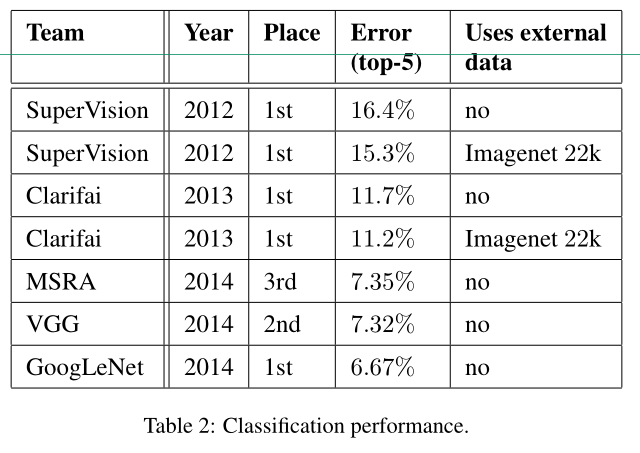
이를 위해 다음 세 가지 실험을 수행했다.

1. stride가 2인 299x299 receptive field를 사용하고, 첫 번째 layer 다음에 max pooling을 사용.

2. stride가 1인 151x151 receptive field를 사용하고, 첫 번째 layer 다음에 max pooling을 사용.

3. stride가 1인 79x79 receptive field를 사용하고, 첫 번째 layer 다음에 pooling layer가 없음.

위 실험에 해당하는 3개의 네트워크는 거의 동일한 계산 비용을 갖는다. 실제로는 3번 네트워크가 약간 저렴하지만, pooling layer의 계산 비용은 총 비용의 1% 이내 수준이기 때문에 무시한다. 각각의 네트워크는 수렴 될 때까지 학습했으며, 성능은 ImageNet ILSVRC 2012 classification benchmark의 validation set에 대해 측정됐다. 결과는 Table.2에서 혹인할 수 있다. lower-resolution networks는  네트워크가 학습하는 데 시간이 오래 걸리긴 하지만, 성능은 higher resolution newwork에 상당히 유사하다. 그러나 input resolution에 따라 단순하게 네트워크 크기를 줄이게 된다면 성능이 훨씬 떨어지게 된다. 하지만, 이는 어려운 작업에 대해서 16배나 저렴한 모델이기 때문에, 이를 비교하는 것은 불공평하다.

또한 Table.2의 결과들은, R-CNN[5] context 의 smaller object에 대해, high-cost low resolution networks 의 사용 가능성을 암시한다.

10. Experimental Results and Comparisons

Table 3은 Section 6에서  설명한 바와 같이 제안된 아키텍처 (Inception-v2) 의 인식 성능에 관한 실험 결과를 보여준다. 각 Inception-v2은 강조 표시된 새로운 modification 과 모든 이전 수정 사항을 포함한 누적된 변경의 결과를 보여준다. Label Smoothing은 Sect. 7에서 설명한 방법이다. Factorized 7 × 7은 first 7 × 7 convolutional layer를 이어 3 × 3 convolutional layers sequence로 인수분해 하는 부분을 포함한다. BN-auxiliary는 auxiliary classifier의 fully connected layer 가 convolutions뿐만 아니라  batch-normalized에도 버전을 말한다. 우리는 Table 3 마지막 줄에 있는 모델을 Inception-v3으로 언급하고 있으며 multi-crop 및 ensemble settings에서 성능을 평가하고 있다.

모든 evaluations 는 [16]에서 제안한 데로 ILSVRC-2012 validation set의 non-blacklisted examples의 48238 예에 대해 수행된다. 우리는 또한 모든 50000 examples를 평가했고 결과는 top-5 error 에서 약 0.1%, top-1 error 떨어졌다.pcoming version 의 이 논문에서 , 우리는 test에 대한 ensemble result 를 검증할 것이지만, spring [7] 에  BN-Inception 에 대한 마지막 평가  시점에 test and validation set erro가 매우 잘 상관되는 경향이 있음을 나타낸다.

11. Conclusions

우리는 convolutional networks를 scale up하기 위한 몇가지 design principles을 제공하고 Inception architecture의 context 에서 연구했다. 이 지침은 단순하고 , 더 monolithic architectures 에 비해 상대적으로 낮은 계산 비용을 가진 고성능 비전 네트워크로 이어질 수 있다. 가장 성능이 좋았던 Inception-v3의 경우, ILSVR 2012 classification에 대한 single-crop 성능이 top-1 error와 top-5 error에서 각각 21.2%, 5.6%에 도달하여 state of the art 기록을 하였다. 

이는 Ioffe et al [7]에서 설명한 네트워크에 비해 계산 비용이 상대적으로 적게 (2.5배) 증가하여 달성되었다.  여전히 우리의 솔루션은 더 denser networks를 기반으로 한 가장 잘 발표된 결과보다 훨씬 적은 계산을 사용한다. 우리의 모델은 계산 비용이 6배 저렴하고 매개 변수를 최소 5배(추정) 적게 사용하면서 He et al[6]의 결과(상위 5개)를 각각 25%(14%) 능가한다. 

4개의 Inception-v3 models 의 ensemble 은 3.5%에 도달하며, multi-crop evaluation 3.5%  의 top-5 error에 도달한다. 이는 best published results 에 대한 25% 이상의 reduction를 나타내며 ILSVRC 2014 winining GoogLeNet ensemble 오류에 거의 절반 해당한다. 

또한, 79x79의 낮은 receptive field resolution에서도 high quality results 을 얻을 수 있음을 입증했다. 이는 상대적으로 작은 object를 탐지하는 시스템에 도움될 수 있다. 이 논문에서는 neural network 에서의 factorizing convolution 기법과 aggressive  dimension reduction으로, 어떻게 높은 성능을 유지하면서도, 비교적 낮은 계산 비용이 드는 네트워크를 만들 수 있는지에 대해 알아봤다. batch-normalized auxiliary classifiers 및 label-smoothing 기법이 함께 사용되면, 크지 않은 규모의 학습 데이터 상에서도, 고성능의 네트워크를 학습 할 수 있다.

논문 출처 :

Rethinking the Inception Architecture for Computer Vision

참고 :

https://sike6054.github.io/blog/paper/third-post/

요즘 파파고도 잘 되어 있어서 파파고 번역을 많이 참고하였다.

https://sike6054.github.io/blog/paper/third-post/

논문 : Identity Mappings in Deep Residual Networks

2016년

Abstract

Deep residual networks 는 매우 deep architectures 으로 등장하여 compelling accuracy and nice convergence behaviors 의 특성을 가지는 것을 알 수 있다.여기에서 우리는 the propagation formulations behind the residual building blocks 분석하며 , which suggest that the forward and backward signals can be directly propagated from one block to any other block, when using identity mappings as the skip connections and after-addition activation. 

일련의 ablation experiments은 these identity mappings에서 중요한 역할을 하는 것을 검증한다. 이것으로 하여 우리는 

a new residual unit를 제안하였으며 , 이 것으로 하여 우리는 학습을 쉽고 일반화를 높일 수 있게 하였습니다.

improved 결과 :

a 1001-layer ResNet on CIFAR-10 (4.62% error) and CIFAR-100 

a 200-layer ResNet on ImageNet.

Code is available at: https://github.com/KaimingHe/ resnet-1k-layers.

1 Introduction

Deep residual networks (ResNets) 은 여러개 “Residual Units” 로 쌓여있는 형태이다. 

F is a residual function.

h(xl) = xl is an identity mapping and f is a ReLU [2] function.

identity mapping : 항등 함수(恒等函數, 영어: identity function) 또는 항등 사상(恒等寫像, 영어: identity map), 항등 변환(恒等變換, 영어: identity transformation)은 정의역과 공역이 같고, 모든 원소를 자기 자신으로 대응시키는 함수이다.

ResNets that are over 100-layer 을 사용하여 우리는 several challenging recognition tasks on ImageNet [3] and MS COCO [4] competitions에서 높은 정확도가 나왔는지 알 수 있다. ResNets의 핵심 사상은 to learn the additive residual function F with respect to h(xl), with a key choice of using an identity mapping h(xl) = xl .이것은 identity skip connection (“shortcut”) 첨가하여 실현하였다.

In this paper, we analyze deep residual networks by focusing on creating a “direct” path for propagating information — not only within a residual unit, but through the entire network. Our derivations reveal that if both h(xl) and f(yl) are identity mappings, the signal could be directly propagated from one unit to any other units, in both forward and backward passes. 우리의 실험 경험적으로 볼 때 , 이 architecture 가 두가지 상태에 가까울 때 , 학습이 좀 더 간단해졌다.

To understand the role of skip connections, we analyze and compare various types of h(xl).

우리는 skip connections 의 역할을 이해하기 위하여 , 우리는 여러가지 타입의 h(xl) 비교하면서 분석하였다. 우리는 identity mapping h(xl) = xl 선택하여 사용해서 우리가 연구한 모든 유형중에서 , 빠른 error reduction과 최저의 training loss among all variants , whereas skip connections of scaling, gating [5,6,7], and 1×1 convolutions all lead to higher training loss and error. 이들 실험 제안으로 , that keeping a “clean” information path (indicated by the grey arrows in Fig. 1, 2, and 4) is helpful for easing optimization.

an identity mapping f(yl) = yl 구조를 위하여 , 우리는 the activation functions (ReLU and BN [8]) as “pre-activation” ” of the weight layers, conventional wisdom of “post-activation”와 대조하다. 이 점을 통하여 우리는 새로운 residual unit 이 설계되여서 , shown in (Fig. 1(b)). 이 unit을 기존으로 , 우리는 we present competitive results on CIFAR-10/100 with a 1001-layer ResNet, 이것은 많이 쉽게 학습과 일반적으로 original ResNet 보다 학습하기 좋다. ImageNet using a 200-layer ResNet에 대하여 overfit방식이 나타나서 , 우리는 더 나은 것을 표현하기 위하여 개조한 인터넷 결과를 사용하였다. 결과로 인하여 , 심도있게 학습이 성공의 중요 포인터이고 , 모델의 deep learning 은 아직도 더 큰 dimension of network depth있다. 

2 Analysis of Deep Residual Networks

ResNets는 같은 connecting shape 를 통하여 bloks을 stack building으로 모듈화 아키텍츠를 만든다. 여기에서는 우리는 이 blocks를 "Residual Units"이라고 한다. 

xl : the input feature to the l-th Residual Unit. 

Wl = {Wl,k|1≤k≤K} : a set of weights (and biases) associated with the l-th Residual Unit

K :  the number of layers in a Residual Unit (K is 2 or 3 in [1])

F denotes the residual function, e.g., a stack of two 3×3 convolutional layers in [1] 

function f:  the operation after element-wise addition

f is ReLU 

function h : set as an identity mapping: h(xl) = xl

만약 f 는 also an identity mapping: xl+1 ≡ yl , we can put Eqn.(2) into Eqn.(1) and obtain: 

Recursively (xl+2 = xl+1 + F(xl+1, Wl+1) = xl + F(xl , Wl) + F(xl+1, Wl+1), etc.) we will have:

for any deeper unit L and any shallower unit l.Eqn.(4)는 exhibits some nice properties. (i) The feature xL of any deeper unit L can be represented as the feature xl of any shallower unit l plus a residual function in a form of 

, 이것은 any units L and l 사이에서는 모두 residual fashion특성 을 가지고 있다 . (ii)

Eqn. : 영어에서 변역됨 -Unix문서 레이아웃 도구의 troff제품군의 일부인 eqn 은 인쇄 방정식을 형식화하는 전 처리기입니다.

Eqn.(4) also leads to nice backward propagation properties. loss function을 E으로 표시하고 , from the chain rule of backpropagation [9] we have: 

두가지로 분해 할 수 있다. 

그중에서 앞에것은 직접 신호를 전하고 아무른 weight layers와 관계가 없다. 다른 한가지는 propagates through the weight layers . 앞에것은 신호가 직접 다른 shallower unit l의 전달을 보장해준다. 

이것은 weight가 아무리 작어도 , gradient는 소실하지 않는 현상이 생긴다.

Discussions

Eqn.(4) and Eqn.(5)은 both forward and backward 단계에서 , 신호는 직접 이 unit에서 임의의 다른 unit으로 직접 전달 할 수 있다. 

The foundation of Eqn.(4) is two identity mappings:

(i) the identity skip connection h(xl) = xl

(ii) the condition that f is an identity mapping

이들 directly propagated information flows은 Fig. 1, 2, and 4에서 grey arrows로 표시한 것으로 한다. these grey arrows cover no operations (expect addition) and thus are “clean” 일 경우 , 위의 두가지 조건은 성립된다. 아래의 두 부분에서는 우리는 두가지 조건의 작용에 대하여 갈라서 결과를 연구한다.

3 On the Importance of Identity Skip Connections

간단한 수정을 설계한다. h(xl) = λlxl 으로 to break the identity shortcut: 

λl  :  a modulating scalar (for simplicity we still assume f is identity).

여기서 재귀적으로 지원해서 푼다면 Eqn. (4)와 비슷한 것을 얻는다 :

그중 the scalars into the residual functions를 합친다.  이것은 Eq.5 와 비슷하다. 우리는 backpropagation의 전파 과정은 위의 겉과 같다. 

Eq.5와 같지 않게 , Eq.8중에서 first additive term 은 요소에 따라 변조한다.

극단적인 deep network중에서 (L은 매우 크다) 

만약 λi > 1 for all i : 요소들은 exponentially 클 수 있다.

만약 λi < 1 for all i : 요소들은 exponentially 작아지거나 소실 할 수 있다. which blocks the backpropagated signal from the shortcut and forces it to flow through the weight layers. 우리는 실험을 통해 optimazation 의 우화를 어렵게 할 수 있다는 것을 증명하였다.

위의 분석중 , Eqn.(3)중의 original identity skip connection 은 with a simple scaling h(xl) = λlxl로 대체할 수 있다. 

만약 skip connection h(xl)은 더욱 복잡하게 변형한다는 것을 대표한다면 s (such as gating and 1×1 convolutions), 

in Eqn.(8) the first term 은 방정식으로 표현한다. 이런 성적으로는 똑 같이 information propagation 방해하고 and hamper the training procedure 아래의 실험에서 우리는 익서을 증명할 수 있다. 

Figure 2 Table 1에서의 여러가지 타입의 shortcut 을 연결한다. greay arrow에서는 정보전파의 최단거리를 표시한다 . (b-f)중에서 sortcut연결은 다른 같지 않은 성분으로 방행하였다. 간단하게 할려고, 우리는 BN layers를 그리지 않고 이것은 weight layers의 뒤에 연결해야 한다.

3.1 Experiments on Skip Connections

우리는 110-layer ResNet 에서 CIFAR-10을 사용하였다. 

extremely deep ResNet-110 : 

54 two-layer Residual Units (consisting of 3×3 convolutional layers) 

challenging for optimization

우리의 실험 자세한 정보는 ((see appendix ) are the same as [1]. random variations의 영향을 피하기 위하여 , 여기에서 우리는 5 runs for each architecture on CIFAR 중 median accuracy을 결과로 하였다.

위의 분석중 f는 identity mappeng으로 하였지만 , 여기에서 실험할 경우 f = ReLU으로 모두 하였다 , 다음 부분부터 우리는 identity f 로 분석을 진행한다. 우리의 baseline ResNet-110 는 6.61% error on the test set 가 있다. 다른 variants와 비교하는것은 s (Fig. 2 and Table 1) 에서 요약한것과 같다:

Constant scaling.

모든 shortcuts의 연결중 λ = 0.5 , 우리는 더욱이 F 를 두가지 scaling 으로 고려한다.: 

(i) F is not scaled; => 이 caset는 does not converge well

(ii) F is scaled by a constant scalar of 1−λ = 0.5, which is similar to the highway gating [6,7] but with frozen gates.=> is able to converge, but the test error (Table 1, 12.35%) is substantially higher than the original ResNet-110.

Fig 3(a) shows that the training error is higher than that of the original ResNet-110, suggesting that the optimization has difficulties when the shortcut signal is scaled down.

Exclusive gating. 

Following the Highway Networks [6,7] that adopt a gating mechanism [5], 우리는 gating function을 고려한다. weight, biases, sigmoid함수로 변환하면서 한다. convolutional network g(x)중 1×1 convolutional layer을 통과하여 실현한다. gating 함수는 element-wise 곱하여 신호를 조절한다.

우리는 investigate the “exclusive” gates as used in [6,7] — — the F path is scaled by g(x) and the shortcut path is scaled by 1−g(x).  See Fig 2(c). 우리는 초기화 biase가 중요한 학습 gated의 모듈인것과 가이드라인에 따라 하는 것이 중요하다는 것을  발견하였다.  우리는 bias를 0부터 10 까지를 초기화 범위로 하고 , 하나씩 줄이고 그다음 cross-validation방법을 통해 hyper-parameter을 찾으면서 실행하였다. 그리고 최적 의 갓ㅂ으로 훈련하여 , leading to a test result of 8.70% (Table 1), 그래도 original ResNet-110보다 휠씬 뒤떨어져있다. Fig 3(b)은 훈련과정을 표시한다. Table 1도 다른 초기화 값을 이용하여 실험환 결과를 보여주고 , bg의 초기화 값이 합법적이지 않을 경우 exclusive gating does not converge to a good solution하는것을발견하였다.

exclusive gating mechanism은 two-fold 영향을 받는다. 

1 − g(x) 가 1에 가까울때 ,  the gated shortcut connections are closer to identity  which helps information propagation; =>신호 전달에 도움이 된다.

g(x) approaches 0 and suppresses the function F. To isolate the effects of the gating functions on the shortcut path alone, we investigate a non-exclusive gating mechanism in the next.  

Shortcut-only gating. function F is not scaled; only the shortcut path is gated by 1−g(x). See Fig 2(d). initialized value of bg는 이 case에도 여전히 중요하다.

When the initialized bg is 0 (so initially the expectation of 1 − g(x) is 0.5), the network converges to a poor result of 12.86% (Table 1). This is also caused by higher training error (Fig 3(c)). 낮다. 

When the initialized bg is very negatively biased (e.g., −6), 1−g(x)의 값이 1에 가깝고 and the shortcut connection is nearly an identity mapping. 

1×1 convolutional shortcut. Next we experiment with 1×1 convolutional shortcut connections that replace the identity. 이 선택적 방안은 34-layer ResNet(16 Residual Units)에 사용(option C )하였고 좋은 결과를 가질 뿐만 아니라 ,suggesting that 1×1 shortcut connections could be useful.  하지만 우리는 this is not the case when there are many Residual Units인 것을 발견하였다. 1×1 convolutional shortcuts을 사용할 경우 110-layer ResNet 은 좋지 않은 결과가 나왔다(12.22%, Table 1 ).  Again, the training error becomes higher (Fig 3(d)). stacking so many Residual Units (54 for ResNet-110)일 경우 , the shortest path일지라도 신호 propagation을 방해한다. 우리는 on ImageNet with ResNet-101 when using 1×1 convolutional shortcuts 일 경우 비슷한 결과를 나타났다.

Dropout shortcut. 마지막으로 우리는 dropout [11] (at a ratio of 0.5) which we adopt on the output of the identity shortcut (Fig. 2(f))으로 실험한다 . The network fails to converge to a good solution.  Dropout 통계적으로  imposes a scale of λ with an expectation of 0.5 on the shortcut, and similar to constant scaling by 0.5, 똑같이 signal propagation을 방해한다.

3.2 Discussions

Fig. 2의 회식 arrow중 표시한듯이 , shortcut connections는 정보 전파 중 제일 직접적인 경로이다. 

Multiplicative manipulations (scaling, gating, 1×1 convolutions, and dropout) on the shortcuts can hamper information propagation 과 optimization 문제가 생긴다. 

주목해야 할 점은 the gating and 1×1 convolutional shortcuts은 더 많은 파라미터를 설명하였고 , 

identity shortcuts보다 더 강한 표현 능력이 있어햐 한다. 사실은 shortcut-only gating 와 1×1 convolution over the solution space of identity shortcuts (i.e., they could be optimized as identity shortcuts).  하지만 , their training error 는 identity shortcuts보다 훨씬 높아서 , degradation of these models 을 나타나며 원인은 optimazation issues, 표현 능력의 문제가 아니다 . 

4 On the Usage of Activation Functions

위의 실험내용에서 우리는 Eqn.(5) and Eqn.(8)의 내용에 대해 분석하고 , 두가지 공식은 전부 both being derived under the assumption that the after-addition activation f is the identity mapping. 하지만 위의 실험에서 f is ReLU as designed in [1], so Eqn.(5) and (8) are approximate in the above experiments. 다음에 우리는 f 의 영향에 대해 연구한다.

우리는 re-arranging the activation functions (ReLU and/or BN)을 통하여 f를 identity mapping 으로 하고 싶다. The original Residual Unit 의 모양은 Fig.4(a) 중 처럼 BN은 매 weight layer중 사용하고 그다음 ReLU, 그리고 마지막에 element-wise를 추가하고 마지막에 ReLU(f=f= ReLU)추가한다. Fig.4(b-e)는 우리가 연구한 다른 모양을 해설하였다.

4.1 Experiments on Activation

우리는 ResNet-110 and a 164-layer Bottleneck [1] architecture (denoted as ResNet-164)으로 실험하였다 . A bottleneck Residual Unit 는 1×1 layer for reducing dimension으로 포함되였고 , , a 3×3 layer, and a 1×1 layer for restoring dimension(차원 복원). As designed in [1], 계산 복잡도는 two-3×3 Residual Unit과 비슷하다. 더 자세하게는 in the appendix에 있다.  The baseline ResNet164 has a competitive result of 5.93% on CIFAR-10 (Table 2).

BN after addition. Before turning f into an identity mapping , we go the opposite way by adopting BN after addition (Fig. 4(b)). 이 케이스에서는 f는 BN과 ReLU가 포함되였다. 이 결과는 baseline의 결과보다 훨 낮다(Table2). 원래의 original 설계와 다르게, now BN layer 는 지나가는 경로의 the shortcut 신호를 변하게 하고 정보 propagation을 방해하고 , 이것은 훈련 처음 부터 reducing training loss의 힘드는 것을 보인다(Fig.6 left). 

ReLU before addition. f into an identity mapping 의 소박한 선택은 ReLU를 Addition 전으로 이동한다(Fig. 4(c)).하지만 , the transform F의 output이 non-negative으로 하고 , while intuitively a “residual” function should take values in (−∞, +∞). 이 결과를 얻는 이유는 he forward propagated signal is monotonically increasing . 이것은 표현 능력에 영향을 주고 , 결과를 baseline보다 더욱 나쁘게 한다(7.84%, Table 2).  우리는 잔차함수가 (−∞, +∞)의 값 사이에 있기를 희망한다. 이 조건은 n is satisfied by other Residual Units including the following ones.

원래의 설계중 , 활성화 함수는 두가지 길에서 다음희 Residual Unit에서 영향을 준다.

그다음 우리는 asymmetric 방식을 연구

notation에 재명명을 통하여 우리는 위의 공식 형식을 얻을 수 있다. 

우리는 쉽게 Eqn.(9) 과 Eqn.(4) 비슷하다는 것을 알 수 있어서  , 그래서 우리는 a backward formulation similar to Eqn.(5)을 얻을 수 있다. For this new Residual Unit as in Eqn.(9),  he new after-addition activation는 an identity mapping을 으로 되였다. 이 설계의 의미는 

post-activation/pre-activation 사이의 차이는 the presence of the element-wise addition가 원인이다. For a plain network that has N layers, there are N − 1 activations (BN/ReLU), and it does not matter whether we think of them as post- or pre-activations. 하지만 우리가 추가한 branch layer으로 말하면 , the position of activation matters.

우리는 아래의 두가지 설계를 사용하여 실험을 진행하였다:

(i) ReLU-only pre-activation (Fig. 4(d)), and (ii) full pre-activation (Fig. 4(e)) where BN and ReLU are both adopted before weight layers. Table 2는 the ReLU-only pre-activation performs와 the baseline on ResNet-110/164 비슷하다는 것을 표시하였다. 이 ReLU layer는 BN layer과 연결하여 사용하지 않아서 , 그래서 may not enjoy the benefits of BN [8].

하지만 놀랍게도 , 우리가 BN과 ReLU가 pre-activation을 다 사용할 경우, 그 결과는 improved by healthy margins (Table 2 and Table 3). In Table 3 we report results using various architectures: (i) ResNet-110, (ii) ResNet-164, (iii) a 110-layer ResNet architecture in which each shortcut skips only 1 layer (i.e.,a Residual Unit has only 1 layer), denoted as “ResNet-110(1layer)”, and (iv) a 1001-layer bottleneck architecture that has 333 Residual Units (111 on each feature map size), denoted as “ResNet-1001”. We also experiment on CIFAR100.Table 3 에서 우리의 “pre-activation” models 은 일관되게 baseline counterparts의 보다 좋다. 분석 과정은 아래와 같다. 

4.2 Analysis

우리는 pre-activation의 영향은 두가지를 가지고 있는 것을 발견하였다.

첫째 , f는 identity mapping 이기 때문에 the optimization is further eased (comparing with the baseline ResNet) 

둘째 , using BN as pre-activation improves regularization of the models.

Ease of optimization. 우리는 1001-layer ResNet 을 훈련한 경우 매우 선명하게 영향을 가지고 있다. Fig. 1 shows the curves. original design in [1]을 사용하여 , training error는 처음에 훈련할 경우 매우 천천히 줄어든다. for f=f= ReLU, 만약 negative일 경우 신호는 방해되고 , 그리고 여러가지 Residual Units이 있을 경우 , this effect becomes prominent and Eqn.(3) (so Eqn.(5)) is not a good approximation. 다른 한편으로는 f가 identity mapping 일 경우 , 신호는 can be propagated directly between any two units. 우리의 1001-layer network는 training loss를 낮추는데 매우 빠르다(Fig.1).

It also achieves the lowest loss among all models we investigated, suggesting the success of optimization.

We also find that the impact of f = ReLU is not severe when the ResNet has fewer layers (e.g., 164 in Fig. 6(right)). beginning of training 에서 training curve 는 조금만 영향을 가지는 것 같지만 , 하지만 goes into a healthy status soon. 모니터링을 통해 우리는 관찰되였는데, 원인은 일정한 훈련을 통해,  the weights are adjusted into a status such that yl in Eqn.(1) is more frequently above zero and f does not truncate it (xl is always non-negative due to the previous ReLU, so yl is below zero only when the magnitude of F is very negative).The truncation, however, is more frequent when there are 1000 layers.

Reducing overfitting. Another impact of using the proposed pre-activation unit is on regularization, as shown in Fig. 6 (right). The pre-activation version reaches slightly higher training loss at convergence, but produces lower test error. 이 현상은 on ResNet-110, ResNet-110(1-layer), and ResNet-164 on both CIFAR-10 and 100에서 관찰 할 수 있다. 이것은 아마도 BN’s regularization effect [8]이 원인이다. In the original Residual Unit (Fig. 4(a)), BN normalizes 는 신호이지만 , this is soon added to the shortcut and thus the merged signal is not normalized. 이 빙정규화 신호는 또 다음의 weight layers의 입력에 의해 사용된다. . On the contrary, in our pre-activation version, all weight layers 의 입력은 normalized로 되여있다. 

5 Results

Comparisons on CIFAR-10/100.. Table 4  에서 CIFAR-10/100를 최근의 잴 좋은 방법으로 비교하여 , 우리의 모델 은 매우 경쟁성이 있는 결과를 얻었다. 우리는 these small datasets 에 대해서 , 우리는 특별하게 tailor the network width or filter sizes 할 필요 없고 , 정규화 기술을 사용(such as dropout)할 필요 없이 모델의 효과를 보장하였다. 우리는 단지 간단하고 효과있는 방식을 통하여 -------- going deeper. 이것들의 결과는 demonstrate the potential of pushing the limits of depth.

Comparisons on ImageNet.  다음에 우리는 1000- class ImageNet dataset [3]에서 실험결과를 보여준다. We have done preliminary experiments using the skip connections studied in Fig. 2 & 3 on ImageNet with ResNet-101 [1], and observed similar optimization difficulties. The training error of these non-identity shortcut networks is obviously higher than the original ResNet at the first learning rate(similar to Fig. 3), 자원이 한정되여있어서 우리는 절반을 학습하기로 결정하였다. 하지만 우리는 “BN after addition” version (Fig. 4(b)) of ResNet-101 on ImageNet and observed higher training loss and validation error을 완성하였다. This model’s single-crop (224×224) validation error is 24.6%/7.5%, vs. the original ResNet101’s 23.6%/7.1%. 이것은 Fig. 6 (left)에서 CIFAR의 결과와 같다. 

Table 5는 the results of ResNet-152 [1] and ResNet-2003 을 표시하며 , 전부 처음 부터 학습하였다. We notice that the original ResNet paper [1] trained the models using scale jittering with shorter side s ∈ [256, 480], and so the test of a 224×224 crop on s = 256 (as did in [1]) is negatively biased. Instead, we test a single 320×320 crop from s = 320, for all original and our ResNets. Even though the ResNets are trained on smaller crops, they can be easily tested on larger crops because the ResNets are fully convolutional by design. This size is also close to 299×299 used by Inception v3 [19], allowing a 공평한 비교이다.

The original ResNet-152 [1] has top-1 error of 21.3% on a 320×320 crop, and our pre-activation counterpart has 21.1%. The gain is not big on ResNet-152 because this model has not shown severe generalization difficulties.하지만 original ResNet-200 의 error rate of 21.8%이고 , baseline ResNet-152보다 높다. . But we find that the original ResNet-200 has lower training error than ResNet-152, suggesting that it suffers from overfitting.

우리의 pre-activation ResNet-200 의 error rate는 20.7%, which is 1.1% lower than the baseline ResNet-200 and also lower than the two versions of ResNet-152. When using the scale and aspect ratio augmentation of [20,19], our ResNet-200 has a result better than Inception v3 [19] (Table 5). Concurrent with our work, an Inception-ResNet-v2 model [21] achieves a single-crop result of 19.9%/4.9%. We expect our observations and the proposed Residual Unit will help this type and generally other types of ResNets.

Computational Cost. 우리의 모델의 계산복잡도와 depth는 linear관계를 가진다(so a 1001-layer net is ∼10× complex of a 100-layer net). On CIFAR, ResNet-1001 takes about 27 hours to train on 2 GPUs; on ImageNet, ResNet200 takes about 3 weeks to train on 8 GPUs (on par with VGG nets [22]).

6 Conclusions

이 paper에서는 the propagation formulations behind the connection mechanisms of deep residual networks을 여구하였다. Our derivations imply that identity shortcut connections and identity after-addition activation are essential for making information propagation smooth. 제거 실험(Ablation experiments) demonstrate phenomena that are consistent with our derivations. 우리는 동시에 1000-layer deep networks을 제안하여  that can be easily trained and achieve improved accuracy.

Appendix: Implementation Details

The implementation details and hyperparameters are the same as those in [1]. On CIFAR we use only the translation and flipping augmentation in [1] for training. learning rate는 0.1부터 시작하여, and is divided by 10 at 32k and 48k iterations. Following [1], for all CIFAR experiments we warm up the training by using a smaller learning rate of 0.01 at the beginning 400 iterations and go back to 0.1 after that, although we remark that this is not necessary for our proposed Residual Unit. The mini-batch size is 128 on 2 GPUs (64 each), the weight decay is 0.0001, the momentum is 0.9, and the weights are initialized as in [23].

On ImageNet, we train the models using the same data augmentation as in [1]. The learning rate starts from 0.1 (no warming up), and is divided by 10 at 30 and 60 epochs. The mini-batch size is 256 on 8 GPUs (32 each). The weight decay, momentum, and weight initialization are the same as above.

When using the pre-activation Residual Units (Fig. 4(d)(e) and Fig. 5), we pay special attention to the first and the last Residual Units of the entire network. For the first Residual Unit (that follows a stand-alone convolutional layer, conv1), we adopt the first activation right after conv1 and before splitting into two paths; for the last Residual Unit (followed by average pooling and a fullyconnected classifier), we adopt an extra activation right after its element-wise addition. These two special cases are the natural outcome when we obtain the pre-activation network via the modification procedure as shown in Fig. 5.

[논문 출처] : 

Identity Mappings in Deep Residual Networks

참조:

https://kangbk0120.github.io/articles/2018-01/identity-mapping-in-deep-resnet

https://ko.wikipedia.org/wiki/%ED%95%AD%EB%93%B1_%ED%95%A8%EC%88%98

https://en.wikipedia.org/wiki/Eqn_(software)

https://blog.csdn.net/wspba/article/details/60750007

논문 : Deep Networks with Stochastic Depth

Abstract.

Very deep convolutional networks with hundreds of layers 는 competitive benchmarks에서 오류를 크게 감소 할 수 있습니다. Although the unmatched expressiveness of the many layers can be highly desirable at test time, training very deep networks comes with its own set of challenges. 하지만 여러 가지 문제점이 있다. 

1). gradients can vanish,

2). the forward flow often diminishes

3). the trainning time can be painfully slow

이를 해결하기 위해 우리는 stochastic depth, a training procedure that enables the seemingly contradictory setup to train short networks and use deep networks at test time. 

여기에서 우리는 먼저 very deep networks  시작하고 여러개의 mini-batch로 학습하며 , randomly drop a subset of layers and bypass them with the identify function. 이 간단한 접근으로 보완하여 최근의 resisual networks에 성공하였다. training time의 시간을 줄이고 대체로  거의 모든 data sets에서 테스트 오류를 크게 개선하여 평가에 사용합니다. With stochastic depth 우리는 the depth of residual networks의 층을 늘일 수 있고  even beyond 1200 layers and still yield meaningful improvements in test error (4.91% on CIFAR-10).

1 Introduction

Convolutional Neural Networks (CNNs) 

computer vision [3, 4, 5, 6, 7, 8]

AlexNet had 5 convolutional layers [1]

VGG network and GoogLeNet in 2014 had 19 and 22 layers respectively [5, 7]

ResNet architecture featured 152 layers [8]

computer vision: 컴퓨터 비전(Computer Vision)은 기계의 시각에 해당하는 부분을 연구하는 컴퓨터 과학의 최신 연구 분야 중 하나이다.

Network depth is a major determinant of model expressiveness, both in theory [9, 10] and in practice [5, 7, 8]. However, very deep models also introduce new challenges: vanishing gradients in backward propagation, diminishing feature reuse in forward propagation, and long training time.

determinant :행렬식 : 선형대수학에서 , 행렬식은 정사각 행렬에 스칼라를 대응시키는 함수의 하나이다. 

Vanishing Gradients is a well known nuisance in neural networks with many layers [11].As the gradient information is back-propagated, repeated multiplication or convolution with small weights renders the gradient information ineffectively small in earlier layers. Several approaches exist to reduce this effect in practice, for example through careful initialization [12], hidden layer supervision [13], or, recently, Batch Normalization [14].

Diminishing feature reuse during forward propagation (also known as loss in information flow [15]) refers to the analogous problem to vanishing gradients in the forward direction. gradient 훈련하기 힘들다 . making it hard for later layers to identify and learn “meaningful” gradient directions. Recently, several new architectures attempt to circumvent this problem through direct identity mappings between layers, which allow the network to pass on features unimpededly from earlier layers to later layers [8, 15].

Long training time is a serious concern as networks become very deep.gpu를 사용해도  시간이 오래 걸린다.

The researcher is faced with an inherent dilemma:

shorter networks have the advantage that information flows efficiently forward and backward, and can therefore be trained effectively and within a reasonable amount of time. However, they are not expressive enough to represent the complex concepts that are commonplace in computer vision applications. 효율성

Very deep networks have much greather model complexity, but are very difficult to train in practice and require a lot of time and patience. 시간이 오래 걸린다.

In this paper, we propose deep networks with stochastic depth, a novel training algorithm that is based on the seemingly contradictory insight that ideally we would like to have a deep network during testing but a short network during training. We resolve this conflict by creating deep Residual Network [8] architectures (with hundreds or even thousands of layers) with sufficient modeling capacity; however, during training we shorten the network significantly by randomly removing a substantial fraction of layers independently for each sample or mini-batch. The effect is a network with a small expected depth during training, but a large depth during testing. Although seemingly simple, this approach is surprisingly effective in practice.

stochastic depth substantially reduces training time and test error (resulting in multiple new records to the best of our knowledge at the time of initial submission to ECCV).The reduction in training time can be attributed to the shorter forward and backward propagation, so the training time no longer scales with the full depth, but the shorter expected depth of the network.

We attribute the reduction in test error to two factors: 1) shortening the (expected) depth during training reduces the chain of forward propagation steps and gradient computations, which strengthens the gradients especially in earlier layers during backward propagation; 2) networks trained with stochastic depth can be interpreted as an implicit ensemble of networks of different depths, mimicking the record breaking ensemble of depth varying ResNets trained by He et al. [8].

similar to Dropout [16], training with stochastic depth acts as a regularizer, even in the presence of Batch Normalization [14]. On experiments with CIFAR-10, we increase the depth of a ResNet beyond 1000 layers and still obtain significant improvements in test error.

2 Background

수많은 시도하에서 very deep networks 학습을 올릴 수 있었다. 

Earlier works adopted greedy layer-wise training or better initialization schemes to alleviate the vanishing gradients and diminishing feature reuse problems [12, 17, 18].

주목할 만한 최근의 공헌으로는 very deep networks의 학습은 Batch Normalization을 이용한다.

Batch Normalization 는 which standardizes the mean and variance of hidden layers with respect to each mini-batch.

이 접근으로는 vanishing gradients problem을 줄일 수 있고 yields a strong regularizing effect.

최근에는 몇명의 저자들이  extra skip connections to improve the information flow during forward and backward propagation을 소계하였다. Highway Networks [15] allow earlier representations to flow unimpededly to later layers through parameterized skip connections known as “information highways”, which can cross several layers at once. The skip connection parameters, learned during training, control the amount of information allowed on these “highways”.

Residual networks (ResNets)[8] simplify Highway Networks by shortcutting (mostly) with identity functions.이것은 잴인 단순화하면서 잴 효과가 좋게 학습 효율을 높이며 enables more direct feature reuse. ResNets are motivated by the observation that neural networks tend to obtain higher training error as the depth increases to very large values.This is counterintuitive, as the network gains more parameters and therefore better function approximation capabilities.

The authors conjecture that the networks become worse at function approximation because the gradients and training signals vanish when they are propagated through many layers. => 여러 layers 을 통과할때 

As a fix, they propose to add skip connections to the network.

Dropout. multiplies each hidden activation by an independent Bernoulli random variable.Intuitively, Dropout reduces the effect known as “coadaptation” of hidden nodes collaborating in groups instead of independently producing useful features; it also makes an analogy with training an ensemble of exponentially many small networks. Many follow up works have been empirically successful, such as DropConnect [20], Maxout [21] and DropIn [22].

with different depths, possibly achieving higher diversity among ensemble members than ensembling those with the same depth. Different from Dropout, we make the network shorter instead of thinner, and are motivated by a different problem. Anecdotally, Dropout loses effectiveness when used in combination with Batch Normalization [14, 23]. Our own experiments with various Dropout rates (on CIFAR-10) show that Dropout gives practically no improvement when used on 110-layer ResNets with Batch Normalization.

We view all of these previous approaches to be extremely valuable and consider our proposed training with stochastic depth complimentary to these efforts.

we show that training with stochastic depth is indeed very effective on ResNets with Batch Normalization.

3 Deep Networks with Stochastic Depth

stochastic depth 학습을 할 때는 간단한 직관을 기초로 한다. 학습을 할때 length of a neural network 효울성을 낮추기 위해서는 우리는 랜덤으로 skip layers entirely. 

skip connections

connection pattern is randomly altered for each minibatch. 

For each mini-batch we randomly select sets of layers and remove their corresponding transformation functions, only keeping the identity skip connection. Throughout, 우리는 He et al.가 묘사한 이 아키텍처를 사용한다. 왜냐하면 이 아케텍처는 원래 skip connections가 포함되여있고 it is straightforward to modify, and isolates the benefits of stochastic depth from that of the ResNet identity connections. Next we describe this network architecture and then explain the stochastic depth training procedure in detail.

Conv and BN stand for Convolution and Batch Normalization respectively. This construction scheme is adopted in all our experiments except ImageNet, for which we use the bottleneck block detailed in He et al. [8]. Typically, there are 64, 32, or 16 filters in the convolutional layers (see Section 4 for experimental details).

Conv-BN-ReLU-Conv-BN 

Stochastic depth aims to shrink the depth of a network during training, while keeping it unchanged during testing. We can achieve this goal by randomly dropping entire ResBlocks during training and bypassing their transformations

Bernoulli random variable : 

베르누이 분포(Bernoulli Distribution)는 확률 이론 및 통계학에서 주로 사용되는 이론으로, 스위스의 수학자 야코프 베르누이의 이름에 따라 명명되었다. 베르누이 분포는 확률론과 통계학에서 매 시행마다 오직 두 가지의 가능한 결과만 일어난다고 할 때, 이러한 실험을 1회 시행하여 일어난 두 가지 결과에 의해 그 값이 각각 0과 1로 결정되는 확률변수 X에 대해서

를 만족하는 확률변수 X가 따르는 확률분포를 의미하며, 이항 분포의 특수한 사례에 속한다.

Implicit model ensemble. In addition to the predicted speedups, we also observe significantly lower testing errors in our experiments, in comparison with ResNets of constant depth. One explanation for our performance improvements is that training with stochastic depth can be viewed as training an ensemble of ResNets implicitly. Each of the L layers is either active or inactive, resulting

From the model ensemble perspective, the update rule (5) can be interpreted as combining all possible networks into a single test architecture, in which each layer is weighted by its survival probability.

4 Results

We empirically demonstrate the effectiveness of stochastic depth on a series of benchmark data sets: CIFAR-10, CIFAR-100 [1], SVHN [31], and ImageNet [2].

construction scheme (for constant and stochastic depth) as described by He et al. [8]. In the case of CIFAR-100 we use the same 110-layer ResNet used by He et al. [8] for CIFAR-10, except that the network has a 100-way softmax output. Each model contains three groups of residual blocks that differ in number of filters and feature map size, and each group is a stack of 18 residual blocks. The numbers of filters in the three groups are 16, 32 and 64, respectively. For the transitional residual blocks, i.e. the first residual block in the second and third group, the output dimension is larger than the input dimension. Following He et al. [8], we replace the identity connections in these blocks by an average pooling layer followed by zero paddings to match the dimensions. Our implementations are in Torch 7 [32]. The code to reproduce the results is publicly available on GitHub at https://github.com/yueatsprograms/Stochastic_Depth.

CIFAR-10.

dataset of 32-by-32 color images 

10 classes of natural scene objects 

The training set and test set contain 50,000 and 10,000 images, respectively We hold out 5,000 images as validation set, and use the remaining 45,000 as training samples.Horizontal flipping and translation by 4 pixels are the two standard data augmentation techniques adopted in our experiments, following the common practice [6, 13, 20, 21, 24, 26, 30].

The baseline ResNet is trained with SGD for 500 epochs, with a mini-batch size 128.

The initial learning rate is 0.1, and is divided by a factor of 10 after epochs 250 and 375.

weight decay of 1e-4, momentum of 0.9, and Nesterov momentum [33] with 0 dampening, as suggested by [34].

For stochastic depth, the network structure and all optimization settings are exactly the same as the baseline. All settings were chosen to match the setup of He et al. [8].

The results are shown in Table 1. 

ResNets trained with stochastic depth yield a further relative improvement of 18% and result in 5.25% test error. To our knowledge this is significantly lower than the best existing single model performance (6.05%) [30] on CIFAR-10 prior to our submission, without resorting to massive data augmentation [6, 25].1 Fig. 3 (left) shows the test error as a function of epochs. The point selected by the lowest validation error is circled for both approaches. We observe that ResNets with stochastic depth yield lower test error but also slightly higher fluctuations (presumably due to the random depth during training).

CIFAR-100. Similar to CIFAR-10 color images with the same train-test split, but from 100 classes. 

For both the baseline and our method, the experimental settings are exactly the same as those of CIFAR-10. The constant depth ResNet yields a test error of 27.22%, which is already the state-of-the-art in CIFAR-100 with standard data augmentation. Adding stochastic depth drastically reduces the error to 24.98%, and is again the best published single model performance to our knowledge (see Table 1 and Fig. 3 right).

We also experiment with CIFAR-10 and CIFAR-100 without data augmentation. ResNets with constant depth obtain 13.63% and 44.74% on CIFAR-10 and CIFAR-100 respectively. Adding stochastic depth yields consistent improvements of about 15% on both datasets, resulting in test errors of 11.66% and 37.8% respectively.

SVHN. The format of the Street View House Number (SVHN) [31] dataset that

32-by-32 colored images of cropped out house numbers from Google Street View.

The task is to classify the digit at the center.

There are 73,257 digits in the training set, 26,032 in the test set and 531,131 easier samples for additional training. Following the common practice, we use all the training samples but do not perform data augmentation. For each of the ten classes, we randomly select 400 samples from the training set and 200 from the additional set, forming a validation set with 6,000 samples in total. We preprocess the data by subtracting the mean and dividing the standard deviation. Batch size is set to 128, and validation error is calculated every 200 iterations.

Our baseline network has 152 layers. It is trained for 50 epochs with a beginning learning rate of 0.1, divided by 10 after epochs 30 and 35. The depth and learning rate schedule are selected by optimizing for the validation error of the baseline through many trials. This baseline obtains a competitive result of 1.80%. However, as seen in Fig. 4, it starts to overfit at the beginning of the second phase with learning rate 0.01, and continues to overfit until the end of training. With stochastic depth, the error improves to 1.75%, the second-best published result on SVHN to our knowledge after [30].

Training time comparison. We compare the training efficiency of the constant depth and stochastic depth ResNets used to produce the previous results. Table 2 shows the training (clock) time under both settings with the linear decay rule pL = 0.5. Stochastic depth consistently gives a 25% speedup, which confirms our analysis in Section 3. See Fig. 8 and the corresponding section on hyper-parameter sensitivity for more empirical analysis.

Training with a 1202-layer ResNet. He et al. [8] tried to learn CIFAR10 using an aggressively deep ResNet with 1202 layers. As expected, this extremely deep network overfitted to the training set: it ended up with a test error of 7.93%, worse than their 110- layer network. We repeat their experiment on the same 1202-layer network, with constant and stochastic depth. We train for 300 epochs, and set the learning rate to 0.01 for the first 10 epochs to “warm-up” the network and facilitate initial convergence, then restore it to 0.1, and divide it by 10 at epochs 150 and 225.

The results are summarized in Fig. 4 (right) and Fig. 5. Similar to He et al. [8], the ResNets with constant depth of 1202 layers yields a test error of 6.67%, which is worse than the 110-layer constant depth ResNet. In contrast, if trained with stochastic depth, this extremely deep ResNet performs remarkably well. We want to highlight two trends: 1) Comparing the two 1202-layer nets shows that training with stochastic depth leads to a 27% relative improvement; 2)

ImageNet.

The ILSVRC 2012 classification dataset consists of 1000 classes of images, in total 1.2 million for training, 50,000 for validation, and 100,000 for testing. Following the common practice, we only report the validation errors. We follow He et al. [8] to build a 152-layer ResNet with 50 bottleneck residual blocks. When input and output dimensions do not match, the skip connection uses a learned linear projection for the mismatching dimensions, and an identity transformation for the other dimensions. Our implementation is based on the github repository fb.resnet.torch [34], and the optimization settings are the same as theirs, except that we use a batch size of 128 instead of 256 because we can only spread a batch among 4 GPUs (instead of 8 as they did).

We train the constant depth baseline for 90 epochs (following He et al. and the default setting in the repository) and obtain a final error of 23.06%. With stochastic depth, we obtain an error of 23.38% at epoch 90, which is slightly higher. We observe from Fig.6 that the downward trend of the validation error with stochastic depth is still strong, and from our previous experience, could benefit from further training. Due to the 25% computational saving, we can add 30 epochs (giving 120 in total, after decreasing the learning rate to 1e-4 at epoch 90), and still finish in almost the same total time as 90 epochs of the baseline. This reaches a final error of 21.98%. We have also kept the baseline running for 30 more epochs. This reaches a final error of 21.78%.

Because ImageNet is a very complicated and large dataset, the model complexity required could potentially be much more than that of the 152-layer ResNet [35]. In the words of an anonymous reviewer, the current generation of models for ImageNet are still in a different regime from those of CIFAR. Although there seems to be no immediate benefit from applying stochastic depth on this particular architecture, it is possible that stochastic depth will lead to improvements on ImageNet with larger models, which the community might soon be able to train as GPU capacities increase.

5 Analytic Experiments

we provide more insights into stochastic depth by presenting a series of analytical results. We perform experiments to support the hypothesis that stochastic depth effectively addresses the problem of vanishing gradients in backward propagation. Moreover, we demonstrate the robustness of stochastic depth with respect to its hyper-parameter.

Fig. 7 shows the mean absolute values of the gradients. The two large drops indicated by vertical dotted lines are due to scheduled learning rate division. It can be observed that the magnitude of gradients in the network trained with stochastic depth is always larger, especially after the learning rate drops. This seems to support out claim that stochastic depth indeed significantly reduces the vanishing gradient problem, and enables the network to be trained more effectively. Another indication of the effect is in the left panel of Fig. 3, where one can observe that the test error of the ResNets with constant depth approximately plateaus after the first drop of learning rate, while stochastic depth still improves the performance even after the learning rate drops for the second time. This further supports that stochastic depth combines the benefits of shortened network during training with those of deep models at test time.

6 Conclusion In this paper we introduced deep networks with stochastic depth, a procedure to train very deep neural networks effectively and efficiently. Stochastic depth  reduces the network depth during training in expectation while maintaining the full depth at testing time. Training with stochastic depth allows one to increase the depth of a network well beyond 1000 layers, and still obtain a reduction in test error. Because of its simplicity and practicality we hope that training with stochastic depth may become a new tool in the deep learning “toolbox”, and will help researchers scale their models to previously unattainable depths and capabilities.

[논문출처] : Deep Networks with Stochastic Depth

[출처]:

https://ko.wikipedia.org/wiki/%ED%96%89%EB%A0%AC%EC%8B%9D

https://ko.wikipedia.org/wiki/%EB%B2%A0%EB%A5%B4%EB%88%84%EC%9D%B4_%EB%B6%84%ED%8F%AC

https://ko.wikipedia.org/wiki/%EC%BB%B4%ED%93%A8%ED%84%B0_%EB%B9%84%EC%A0%84

논문 : Going Deeper with Convolutions

NIN 

inception

auxiliary classifier

optimal sparse structure :

1. 다른 Receptive filed를 사용

2. convolution 1, 3, 5 (patch-alignment issues)

3. pooling

4. higher layer로 갈수록 3x3 혹은 5x5 convolution의 비율이 증가해야 함을 암시한다.

Abstract

우리는 ImageNet Large-Scale Visual Recognition Challenge 2014 (ILSVRC14)에서 classification and detection 새로운 state of the art 달성하는   deep convolutional neural network architecture codenamed Inception 을 제안했다. 이 architecture 의 주요 특징은 network 내부의 computing resources의 활용도 향상이다. 세심하게 crafted design에 의해 , 계산 비용을 유지하면서, network 의  depth and width 을 놀렸다. 품질을 최적화하기 위해, architectural decisions 은 Hebbian 와 multi-scale processing의 직관성에 기반으로 했다. ILSVRC14 에 대한 제출에 사용된 모델은 GoogLeNet으로, 22 layers deep network이며 그 품질은 classification and detection의 context에서 평가된다. 

Hebbian principle : 벨을 흔들고 , 강자지 한테 먹는 것을 준다. 오래되면  강아지는 벨 소리를 들으면 저절로 침이 나온다.

1. Introduction

지난 3년 동안, deep learning and convolutional networks [10]의 발전으로 인해, object classification and detection이 크게 향상되었다. 한가지 격려의 뉴스는 이러한 발전의 대부분이 더 powerful hardware, larger datasets and bigger models일 뿐만 아니라 , 주로 새로운 아이디어, 알고리즘 및 향상된 네트워크 아키텍처의 결과라는 것이다. 예를 들어 ILSVRC 2014 competition 의 상위 항목에는 detection purposes으로 동일한 경쟁의 classification dataset세트 외에 데이터 소스가 사용되지 않았다. ILSVRC 2014에 제출한 GoogLeNet 을 실제로 2년 전의 Krizhevsky et al [9]등 winning architecture 보다 12 times fewer parameters사용하면서도 훨씬 더 정확하다. object detection측면에서 가장 큰 이점은 점점 bigger and bigger deep networks의 단순한 적용에서 나온 것이 아니라 Girshick et al [6] 의 R-CNN 알고리즘[6]과 같은 심층 아키텍처와 고전적인 컴퓨터 비전의 시너지에서 나왔다.

또 다른 주목할 만한 요인은 모바일 및 embedded computing의 지속적인 견인으로 알고리즘의 효율성, 특히 성능과 메모리 사용이 증가한다는 것이다. 이 논문에서 제시된 deep architecture 설계로 이어지는 고려사항에는 정확도 수치에 대한 집착보다는 이 요소가 포함되었다는 점이 주목할 만하다. 대부분의 실험에서 추론 시간에 에서 multiply-adds들의  1.5 billion 계산 비용을 유지하도록 설계되었으며, 따라서 모델은 순수한 academic curiosity으로 끝나지 않고 심지어 대규모 데이터셋에서도 합리적인 비용으로 실제 사용할 수 있다.본 논문에서 우리는 컴퓨터 비전을 위한 효율적인 심층 신경망 아키텍처에 초점을 맞출 것이다. 이 architecture의 이름은 Lin et al [12]에서 작성한 Network in network paper이름에서 유래한 것으로 유명한 "“we need to go deeper”" 로 internet meme [1] 과 관련있다. 이름은 Incetpion 이다. => Network in network 

Incetpion "we need to go deeper" 

우리의 경우  “deep”은 두가지 다른 의미로 사용된다. 

1). “Inception module” 의 형태로 새로운 수준의 조직을 도입하고

2). 네트워크 깊이를 증가시킨다는 보다 직접적인 의미에서

일반적으로 사람들은 Arora et al [2]등의 theoretical work에서 영감을 얻고 지침을 얻으면서 Inception model을 [12]의 논리적 장점으로 볼 수 있다. architecture의 이점은 ILSVRC 2014 classification and detection challenges에 대해 실험적으로 증명되었으며, 이는 현재의 state of the art 을 능가한다. 

2. Related Work

LeNet-5 를 시작으로,   convolutional neural networks (CNN) 은 일반적으로  표준구조를 가지고 있다. 즉,  stacked convolutional layers ( 선택적으로 대비 normalization and max-pooling)에 하나 이상의 fully-connected layers가 따라오는 구조 이다. 이러한  기본 구로를 변형한 모델들은 이미지 분류분야에 널리 사용되며, to-data MNIST, CIFAR 및 ImageNet classfication challenge[9, 21] 에서 최고의 성과를 얻었다. ImageNet 과 같은 대용량 데이터에서 최근 trend는 drouput[7] 로 overfitting문제를 해결하면서  레이어 수[12] 와 레이어 사이즈[21,14]를 늘이는 것이다.

max-pooling layers 은 정확한 spatial information을 손실함에서 불구하고 , alexNet[9]와 동일한 convolutional network architecture 가 localization [9, 14], object detection [6, 14, 18, 5] and human pose estimation [19] 에도 성공적으로 사용되였다.

primate visual cortex의 신경과학 모델에서 영감을 받은 Serre et al. [15] multiple scales를 처리하기 위해 크기가 다른 일련의 고정 Gabor filters 를 사용하였다. 우리는 여기서 비슷한 전략을 사용한다. 그러나 [15]의 고정된 2-layer deep mode과 반대로 , Inception architecture 의 필터는 모두 학습된다. 또한 Inception layers은  여러 번 반복되어 GoogLeNet 모델의 경우 22-layer deep model로 이어진다. 

Network-in-Network 는 신경망의 표현력을 높이기 위해 Lin et al. [12] 이 제안한 방식이다. 모델에서 network에 1 × 1 convolutional 을 추가되어 그 깊이가 증가한다. 우리는 아키텍처에서 이 접근 방식을 많이 사용한다.

그러나 우리의 환경에서 1 × 1 convolutions 두가지 목적을 가지고 있다. 

1) . 가장 중요한 것은 그것들은 주로 계산 병목 현상을 제거하기 위한 차원 축소 모듈로 사용되며 

2) . 네트워크의 크기를 제한할 수 있다는 것이다. 

bottlenecks: 병목현상 : 전체 시스템의 성능이나 용량이 하나의 구성 요소로 인해 제한을 받는 현상을 말한다.

이를 통해 성능을 크게 저하시키지 않으면서 , 네트워크의 depth뿐만 아리라  width도 증가시킬 수 있다. 

마지막으로 object detection을 위한 state of the art기술은 Girshick et al.[6] Regions with Convolutional Neural Networks (R-CNN) 방법이다. R-CNN은 전제적인 detection problem두가지 하위 문제로 분해한다. category-agnostic 적인 방식으로 object location proposals을 생성하기 위해 color and texture 와 같은 low-level cues 를 활용하고 CNN classifiers를 사용하여  해당 위치에서 객체 범주를 식별한다. 이러한 2단계 접근방식은 state-of-the-art CNNs의 매우 강력한 classification 뿐만아니라 bounding box segmentation 의 정확성을 활용한다.우리는 detection submissions시 similar pipeline을 채택했지만 higher object bounding box recall을 위한 multi-box [5] prediction및 bounding box proposals의 더 나은  분류를 위한 ensemble approaches 같은 두 단계의 개선사항을 탐구했다.

class-agnostic 탐지기는 객체가 어떠한 분류(class)에 속해 있는지에 대해 구분하지 않고 객체만을 검출하여 bounding box로 인식한다.

ensemble

3. Motivation and High Level Considerations

deep neural networks 의 성능을 향상시키는 가장 간단한 방법은 size를 늘리는 것이다. 여기에는 depth , width 증가 두가지가 포함된다.

1). depth의 증가 - the number of network levers (layer )

2). width의 증가 - the number of units at each level 

이는 특히 대량의 라벨링된 학습데이터를 사용할 수 있는 경우 고품질 모델을 쉽고 안전하게 교육할 수 있는 방법이다. 하지만 간단한 솔루션에는 두가지 주요 단점이 있다.

1). size가 클 수록 parameters의 수가 많아져 확장된 network가 over-fitting되기 쉬우며, 특히 학습 세트에서 라벨링된 예제의 수가 제한적일 경우 더욱 그러하다. 이는 라벨이 강한 데이터 세트를 얻기 어렵고 비용이 많이 들기 때문에 그림 1에서와 같 ImageNet(1000 클래스 ILSVRC 하위 집합에서도)과 같은 다양한 세분화된 시각적 범주를 전문 인간 평가자가 구별해야 하는 주요 병목 현상이다. => verfitting이 되기 쉽기 때문에 세분화한 라벨이 많이 필요하다. 

2).  또 다른 단점은 네트워크의 크기를 늘리는 것은 컴퓨터 자원의 사용이 크게 증가한다.컴퓨터 계산 능력이 크게 요구된다. 예를 들어 , deep vision network에서 두개의 convolutional layers가 체인된 경우, filters 수가 증가하면 계산이 quadratic(예: x^2) 증가하게 된다. 추가된 용량이 비효율적으로 사용될 경우(예: 대부분의 가중치가 0에 가까운 경우) 계산의 많은 부분이 낭비된다. 계산 비용은 항상 한정되기 때문에, 주요 목적이 성능 품질을 높이는 것일지라도 크기를 무분별하게 증가시키는 것보다 컴퓨팅 자원의 효율적인 분배가 선호된다. (컴튜어 자원은 한정하기 때문에 , 네트워크의 사이즈를 늘리는 것 보다 컴퓨팅 자원을 효율적으로 분배하는 것이 더 중요하다.)

이 두 가지 문제를 해결하는 근본적인 방법은 sparsity 을 도입하고 , fully connected layers 를 convolutions내부에서도 layers by the sparse로 대체하는 것이다. 

spare connected : 다 연결되는 것이 아니다. 

fully connected : 다 연결한다. 

biological systems모방하는 것 외에도 , 이것은 또한 Arora et al. [2]의 획기적인 연구로 인해 보다 확고한 이론적 토대를 가질 수 있다. 이들의 주요 결과에 따르면, 데이터 세트의 probability distribution가 크고 very sparse deep neural network에 의해 표현될 수 있는 경우, 이전 계층 활성화의 상관 통계를 분석하고 상관 관계가 높은 출력과 함께 뉴런을 클러스터링하여 optimal network topology 를 계층별로 구성할 수 있다. 엄격한 mathematical 증명은 매우 강한 조건을 요구하지만, 이 진술이 잘 알려진 Hebbian principle-함께 작동되는 뉴런들-  사실은 근본적인 아이디어가 덜 엄격한 조건에서도 실제로 적용 가능하다는 것을 암시한다. 

불행히도,  오늘날의 컴퓨팅 인프라는 non-uniform sparse data structures에 대한 수치 계산에서 매우 비효율적이다. arithmetic operations의 수가 100배 감소하더라도, 검색과 캐시 누락의 오버헤드가 지배할 것이다:  sparse matrices로 전환하는 것은 성과를 거두지 못할 수 있다. 이 격차는 매우 빠른 dense matrix multiplication을 가능하게 하는 꾸준히 개선되고 highly tuned numerical libraries를 사용하여 기본 CPU or GPU hardware[16, 9]의 미세한 세부정보를 함으로써 더욱 확대된다. 또한 non-uniform sparse models은 sophisticated engineering and computing infrastructure이 더 필요하다. 대부분의 현재 vision oriented machine learning systems은 단지 convolutions을 채택함으로써 spatial domain 의 희소성을 활용한다. 그러나 convolutions 은 이전 계층의 patches 에 대해 dense connections의 집합으로 구현된다. ConvNets 의 대칭성을 깨고 학습을 개선하기 위해  [11] 이후 feature dimensions에 랜덤 및 parse connection tables 을 사용해 왔지만, parallel computation을 최적화하기 위해 추세는 [9]와의 완전 연결로 다시 바뀌었다. computer vision 을 위한 현재의 state-of-the-art architectures은 균일한 구조를 가지고 있다. filters 수가 많고 배치 크기가 크기 때문에 dense computation을 효율적으로 할 수 있다.

균등 공간 (Uniform space) : 두 점이 서로 "가까운지" 여부가 주어진 집합이다. 

이는 다음 중간 단계, 즉 이론에서 제안한 대로 filter-level sparsity을 사용하지만 밀도가 높은 행렬에 대한 연산을 활용하여 현재 하드웨어를 활용하는 아키텍처에 대한 희망이 있는지에 대한 의문을 제기한다. => filter-level sparsity dense matricessparse matrix computations (e.g. [3])에 대한 방대한 논문은 sparse matrices을 상대적으로 상대적으로 밀도가 높은 하위 행렬로 클러스터링하는 것이 sparse matrix multiplication에 대한 경쟁적 성능을 제공하는 경향이 있음을 시사한다. (하위 행렬로 ) 가까운 미래에 대한 non-uniform deep-learning architectures의 자동 구축을  위해 유사한 방법이 활용될 것이라고 생각하는 것은 믿기지 않은 일이 아닌 것 같다.

Inception architecture는 [2] for vision networks 에서 암시하는 sparse structure를 비슷하게 하고 dense가 높고 쉽게 사용할 수 있는 구성요소로 가정된 결과를 다루는 sophisticated network topology construction algorithm의 가상 출력을 평가하기 위한 사례 연구로 시작되었다. highly speculative undertaking에도 불구하고, Network in network [12]에 기초한 기준 네트워크와 비교했을 때 초기에 약간의 이득이 관찰되었다. 약간의 뉴닝으로 격차는 더욱 벌어졌고, 인셉션은 [6] 및 [5]의 기본 네트워크로서 localization 및 object detection의 context에서 특히 유용하다는 것이 입증되었다. 흥미롭게도 , 대부분의 초기 아키텍처 선택에 의문을 제기하고 분리하여 철저히 테스트했지만, locally으로 최적에 가까운 것으로 드러났다. 그러나 주의해야 할 것은 nception architecture가 컴퓨터 비전의 성공이 되었지만, 이것이 그것의 구축을 이끈 지침 원리에 기인할 수 있는지는 여전히 의문이라는 점이다. 이것을 확실히 하려면 훨씬 더 철저한 분석과 검증이 필요할 것이다. 

4. Architectural Details

Inception architecture의 주요 아이디어는 convolutional vision network의 최적의 local sparse structure 를 어떻게 근사하고 쉽게 이요할 수 있는 dense components로 구성할 수 있을지를 알아내는 것이다. translation invariance을 가정하면 convolutional building blocks 으로 구축하는 것을 의미한다. 우리가 필요한 것은 local construction 을 찾고 , 그것을 공간적으로  반복하는 것이다. Arora et al. [2] 는 마지막 계층의 상관관계 통계를 분석하여 높은 상관관계를 가진 단위 그룹으로 군집화해야 하는 계층별 구성을 제안한다. 이러한 clusters 는 다음 계층의 단위를 형성하고 이전 계층의 단위에 연결된다. 이전 계층의 각 장치는 입력 이미지의 일부 영역에 해당하며 이러한 장치는 filter banks로 그룹화된다고 가정한다. 하위 계층 (입력 가까이에 있는 계층)에서는 상관된 단위가 로컬 영역에 집중된다. 따라서, 우리는 많은 클러스터가 단일 영역에 집중될 것이고, 그것들은 [12]에서 제시된 바와 같이, 다음 계층의 1×1 컨볼루션 층으로 덮일 수 있다. 그러나 더 큰 패치에서 컨볼루션에 의해 커버될 수 있는 공간적으로 분산된 클러스터가 더 적을 것이며 더 큰 영역에 걸쳐 패치의 수가 줄어들 것으로 기대할 수 있다. (????)  (큰 patch size의 convolution을 사용함으로써, 적은 수의 cluster로도 더 넓게 펼쳐질 수 있으며, 이를 통해 patch의 수가 감소될 수도 있다. Patch는 filter로 생각하면 된다. ) patch-alignment issues를 피하기 위해,  Inception architecture의 구성 요소는 1×1, 3×3 and 5×5로 제한한다. 이 결정은 필요성보다는 편의성에 더 중점을 두었다. 즉 , 제안된 아키텍처가 다음 단계의 입력을 형성하는 a single output vector로 연결된 output filter banks의 모든 layer들의 결합이라는 것을 의미한다. 또한 pooling operations은 현재 convolutional networks의 성공에 필수적으므로 , 그러한 각 단계에서 alternative parallel pooling path 를 추가하는 것도 이점을 가질 수 있다는 것을 암시한다. (see Figure 2(a)).

filter banks : 신호 처리에서 필터 뱅크는 입력 신호를 여러 구성 요소로 분리하는 대역 통과 필터의 배열이며, 각 구성 요소는 원래 신호의 단일 주파수 하위 대역을 전달합니다.  

이런 “Inception modules”모델이 서로 겹쳐 쌓이면 출력의 output correlation statistics가 달라질 수 밖에 없는데, higher abstraction의 특징이 higher layers에 의해 포착되면 간 집중도가 감소할 것으로 예상된다. 이는 3×3과 5×5 컨볼루션의 비율이 더 높은 계층으로 이동함에 따라 증가해야 함을 암시한다. 

위의 모델에서의 한가지 문제점은 naive form 에서 filter 수가 많은 컨볼루션 레이어 위에 적당한 수의 5×5 컨볼루션도 엄청나게 비쌀 수 있다는 것이다. 이 문제는 pooling units이 추가되면 훨씬 더 부각된다. output filters 의 수는  이전 단계의 필터 수와 같다. pooling layer 의 출력과 convolutional layers 출력의 병합은 단계마다 출력의 수의 불가피한 증가를 초래할 것이다. 이 아키텍처는 optimal sparse structure를 포함할 수 있지만, 매우 비효율적으로 수행할 수 있으며, 몇 단계 내에 계산 폭발을 초래할 수 있다.

이것은 인셉션 아키텍처의 두 번째 아이디어로 이어진다. 즉, 계산 요구 사항이 지나치게 증가할 경우 신중하게 차원을 줄이는 것이다. (=> reducing dimension) 이는 임베딩의 성공에 기반을 두고 있다 . low dimensional embeddings에도 많은 정보가 포함될 수 있다, 하지만 embeddings 은  information in a dense가 압축된 형태로 나타내며 압축된 정보는 처리하기가 더 어렵다. 표현은([2]의 조건에 의해 요구되는) 대부분의 장소에서 sparse 하게 유지되어야 하며 신호를 일괄 집계해야 할 때마다 압축해야 한다. 즉 계산량이 많은 3x3이나 5x5 convolution 이전에는 reduction을 위한 1x1 convolution이 사용된다. reduction은 rectified linear activation의 사용함으로써  dual-purpose 으로 활용된다. 최종 결과는 그림 2(b)에 나타나 있다. 

일반적으로 Inception network는 위 유형의 모듈들이 서로 겹쳐져 있는 네트워크이며, grid의 해상도를 절반으로 줄이기 위해 stride 2가 있는 max-pooling layers 를 사용한다. 기술적인 이유(훈련 중 메모리 효율성)로 인해, lower layers 전통적인 convolutional 방식으로 유지하면서 higher layers에서만 사용하는 것이 유익하다. 이

는 엄격하게 필요하지 않으며 단지 현재 구현의 비효율적인 infrastructural 을 고려한 것이다.

이 architecture 의 유용한 측면은 이후의 stage 에서 omputational complexity의 제어되지 않은 blow-up in computational 증가 없이 각 단계에서 unit 수 를 크게 늘릴 수 있다는 것이다. 이는 patch sizes 를 갖는 expensive convolutions 에 앞서 어디에서나 dimensionality reduction를 사용함으로써 달성된다. 또한 디자인은 visual information를 different scales로 처리하고 그 다음 단계가 다른 척도에서 동시에 특징을 추상화할 수 있도록 종합해야 한다는 실용적인 직관을 따른다. 

computational  resources의 사용이 개선되어 , 각 stage 의 width 은 computational 에 빠지지 않게 단계 수를 늘릴 수 있다.

Inception architecture를 사용하여 약간의 열등하지만  계산적으로는 더 저렴한 버전을 만들 수 있다. 우리는 사용 가능한 모든 knobs and levers 를 통해 계산 리소스의 제어된 밸런싱을 허용하여 비인셉션 아키텍처의 유사한 수행 네트워크보다 3~10배 빠른 네트워크를 만들 수 있지만, 이 시점에서 신중한 수동 설계가 필요하다는 것을 발견했다. 

NIN 

컴퓨팅 자원 등 

5. GoogLeNet

“GoogLeNet”이름으로 우리는 ILSVRC 2014 competition submission Inception architecture의 특징 형태를 말한다 . 우리는 약간 우수한 품질의 깊고 넓은 Inception network를 사용했고 그 네트워크는 앙상블에 추가하니 결과만 조금 나아지는 것 같았다. 경험에 따르면 , exact architectural parameters 의 영향은 상대적으로 미미하며, network의 세부 사항은 생략한다. Table 1은 competition에서 가장 흔히 사용되는 인셉션의 예를 보여준다. 이 네트워크(다른 이미지 패치 샘플링 방법으로 훈련됨)는 앙상블의 7개 모델 중 6개 모델에 사용되었다. 

Inception modules 내부를 포함한 모든 convolutions은 rectified linear activation를 사용한다. receptive field의 크기는 the RGB color space with zero mean에서  224×224이다. “#3×3 reduce” 와 “#5×5 reduce” 는 3×3 and 5×5 convolutions 이전에 사용된 reduction layer 1×1 filters를 볼 수 있다. pool proj column에 내장된 max-pooling후 projection layer 에서 1×1 filters를 볼 수 있다. 이 모든 reduction/projection layers은 rectified linear activation도 사용한다.  

네트워크는 계산 효율성과 실용성을 염두에 두고 설계되었으며, 특히 메모리 공간이 적은 계산 자원을 가진 장치를 포함하여 개별 장치에서 추론을 실행할 수 있다.

이 네트워크는 parameters 가 있는 layer만 셀 때 22 layers deep 

pooling까지 계산하면 27 layers이다.

네트워크 구축에 사용되는 전체 계층(independent building blocks) 수는 약 100개이다. exact number는 machine learning infrastructure에 의해 layers 계산하는 방식에 따라 달라진다. 분류기 이전의 평균 풀링의 사용은 [12]에  에 두고 있어나 우리의 구현은 추가적인  linear layer를 가지고 있다.  linear layer를 사용하면 네트워크를 다른 레이블 세트에 쉽게 적응시킬 수 있지만, 주로 편의상 사용되며 큰 효과를 기대할 수 없다. fully connected layers에서 average pooling 사용하면 top-1 정확도를 0.6% 정도 증가했으나 dropout의 중요성은 fully connected layers층이 없음에도 중요한 역할을 보였다. 

linear layer => fully connected layers

네트워크의 비교적 큰 깊이를 고려할 때, gradients 를 효과적으로  모든 계층을 통해 다시 전파할 수 있는 능력이 관심사였다. 이 작업에서 shallower networks의 강력한 성능은 네트워크 중간에 있는 층에 의해 생성된 기능이 매우 차별적이어야 함을 시사한다.이러한 중간 계층에 연결된 auxiliary classifiers를 추가함으로써, 분류기에서 하위 단계의 차별이 예상되었다.  또한, 저자들은 보조 분류기의 추가가 regularization 효과와 함께 vanishing gradient problem를 해결해주는 것으로 생각한다.  이러한 분류기는 인셉션 (4a) 및 (4d) 모듈의 출력 위에 놓인 더 작은 컨볼루션 네트워크의 형태를 취한다. 학습 기간에는 그들의 손실은 할인 가중치로 네트워크의 전체 손실에 더해진다. (보조 분류기의 손실은 0.3으로 가중되었다.) (보조 분류기의 loss는 30%만 고려하고 있다.) 추론 에서는 auxiliary networks를 사용하지 않는다. 이후 control experiments 결과 auxiliary networks의 효과는 상대적으로 미미하며(약 0.5%) 동일한 효과를 달성하는 데 두 네트워크 중 하나만 필요하다는 것이 밝혀졌다.

auxiliary classifier를 포함한 extra network on the side의 정확한 구조는 다음과 같다. 

• filter size  5×5 와 stride 3 인 average pooling layer 출력의 shape은 4×4×512 output for the (4a), and 4×4×528 for the (4d) stage.

• dimension reduction을 위한 1×1 convolution with 128 filters및  rectified linear activation.

• fully connected layer   1024 units 및  rectified linear activation.

• 70% ratio  dropout layer 

•  linear layer 를 사용한 softmax loss as the classifier 1000(predicting the same 1000 classes as the main classifier, but removed at inference time).

결과적으로 얻은 schematic view은 그림 3에 설명되어 있다. 

6. Training Methodology

GoogLeNet 네트워크는 적당한 양의 모델과 데이터 병렬주의를 사용하여 DistBelief[4] 분산 머신러닝 시스템을 사용하여 훈련되었다. CPU based implementation 으로 사용했지만, 대략적인 추정에 따르면 GoogLeNet 네트워크는 일주일 내에 고급 GPU 몇 개를 사용하여 수렴하도록 훈련될 수 있으며, 주요 제한 사항은 메모리 사용량이다. 우리의 학습에서는 asynchronous stochastic gradient descent with 0.9 momentum [17]

fixed learning rate schedule (decreasing the learning rate by 4% every 8 epochs)

을 사용했다. 추론 시간에 사용된 최종 모델을 만들기 위해 Polyak averaging [13]을 사용했다. 

Image sampling방법은 competition의  몇달 동안 크게 변화하였으며, 이미 converged models은 다른 옵션과 함께 학습되었으며, 때로는 dropout  및 learning rate과 같은 hyperparameters를 변화했기도 했다. 따라서 이러한 네트워크를 학습시키는 가장 효과적인 단일 방법에 대한 명확한 지침을 제공하는 것은 어렵다. 상황을 더 복잡하게 만든다면,  일부 모델은 주로 [8]에서 영감을 받아 작은 crop에 대해 주로 학습하였고 , 다른 모델은 더 큰  crop에 대해 학습되었다. 그러나 competition후 매우 잘 작동하는 것으로 확인된 한 가지 처방에는 가로 세로 비율이 간격에 제한된 이미지 영역의 8%와 100% 사이에 크기가 고르게 분포된 이미지의 다양한 크기의 패치 샘플링이 포함된다 [ 3/4,4/3]. ([ 3/4,4/3] 로 제한하여 8%와 100% 크기에서 균등 분포로 patch sampling 하는 것이 매우 잘 동작한다. 다양한 patch의 크기를 사용한다. ) 또한 Andrew Howard[8]의 photometric distortions 이 훈련 데이터의 imaging 조건에 overfitting 하는데 유용하는 것을 발견되였다. 

7. ILSVRC 2014 Classification Challenge Setup and Results

ILSVRC 2014 classification challenge 과제는 Imagenet 에서 1000개의 leaf-node categories에서 하나 선택하는 것이다.

training 1.2 million images

validation 50,000 images

testing 100,000 images

각 이미지는 하나의 ground truth category와 연결되며, 성능은 가장 높은 점수 분류기 예측을 기반으로 측정된다. 두가지 종류의 수치를 본다. 

the top-1 accuracy rate : ground truth가 와 first predicted class비교 

the top-5 error rate : ground truth가 와 first 5 predicted class비교  top-5 개의 class 안에 ground truth가 올바를 경우 순위에 상관 없이 정답이라고 한다. 

대회에서 순위를 할 경우에는 top-5 error rate 을 사용한다. 

우리는 external data를 학습하지 않은 상태로 대회에 참가했다. 본 논문에서 언급한 학습기법 외에도 ,  우리는 더 높은 성능을 얻기 위해 테스트 중에 일련의 기술을 채택했으며, 이 기술은 다음에 설명한다. 

1. 앙상블 - 동일한 GoogLeNet 모델 7개 버전(더 넓은 버전 1개 포함)을 독립적으로 교육하고 앙상블 예측을 수행했다. 각 모델들은 동일한 widht initialization  (감독으로 인해 동일한 초기 가중치를 사용하더라도) 과 learning rate policies학습하였다. 그들은 sampling methodologies와 randomized input image order만 달랐다. 

2. testing동안 우리는 Krizhevsky et al. [9] 그것보다 더 aggressive cropping 자르기 접근법을 채택했다.구체적으로 더 짧은 dimension (height or width) 가 각각 256, 288, 320 및 352인 4개의 scale으로 이미지의 크기를 조정한 다음 크기가 조정된 이미지의 왼쪽, 가운데, 오른쪽 정사각형을 취한다(세로 이미지의 경우 위쪽, 가운데, 아래쪽 정사각형을 취한다). 정 사각형에 대해, 4 corners and the center 224×224 crop 그리고 square resized to 224×224와 조정된 their mirrored versions을 취한다. 이는 이미지당 4×3×6×2 = 144개의 crops로 이어진다. 유사한 접근방식은 전년도의 출품작에서 Andrew Howard[8]에 의해 사용되었으며, 우리는 제안된 계획보다 약간 더 나쁜 성능을 수행하는 것으로 경험적으로 검증했다. 적정한 수의 crops 이 존재하면 더 많은  crops의 이점이 미미해지기 때문에 실제 적용에서는 그러한 공격적인  crops이 필요하지 않을 수 있다는 점에 주목한다.

3. softmax probabilities 은 최종 예측을 얻기 위해 여러 crops과 모든 개별 분류자에 걸쳐 평균화된다. 실험에서 crops에 대한 max pooling  및 분류기에 대한 평균화와 같은 검증 데이터에 대한 대체 접근 방식을 분석했지만, 단순한 평균보다 성능이 떨어진다. 

이 논문의 나머지 부분에서는 최종 성과에 기여하는 여러 요인을 분석한다.

우리의 final submission to the challenges는 검증 및 테스트 데이터 모두에서 상위 5개 오류를 6.67% 얻어 다른 참가자 중 1위를 차지했다. 이는 2012년 SuperVision  접근법에 비해 56.5%의 상대적 감소이며, 두 가지 모두 분류기 교육에 외부 데이터를 사용한 전년도 최우수 접근법(Clarifai)에 비해 약 40%의 상대적 감소이다.Table 2 는 지난 3년간 가장 실적이 좋은 접근법의 통계를

보여준다.

또한 Table 3 에서 이미지를 예측할 때 사용되는 모델 수 와 crops수를 변경하여 여러 테스트 선택의 성능을 분석하고 보고한다. 하나의 모델을 선택할 때, 우리는 validation data에서 가 top-1 error rate 가 잴 낮은 것을 선택했다. 모든 숫자는 testing data statistics에 overfit 되지 않도록 validation dataset에 대해 보고했다.

8. ILSVRC 2014 Detection Challenge Setup and

Results

ILSVRC detection task은 200개의 가능한 클래스 중 이미지의 객체 주위에 경계 상자를 생성하는 것이다. 감지된 객체가 ground truth 와 class 일치 bounding boxes overlap by at least 50%이 되는 경우에 정답인 것으로 계산된다. 관련 없는 검출은 잘못된 긍정으로 계산되고 penalized을 받는다.  classification task와 반대로 , 각 이미지에는 많은 개체가 포함되어 있거나 개체가 없을 수 있으며 그 크기는 다를 수 있다. 결과는 평균 평균 정밀도(mAP)를 사용하여 보고된다. GoogLeNet이 감지를 위해 취하는 접근 방식은 [6]의 R-CNN과 유사하지만, 영역 분류기로 인셉션 모델을 통해 강화된다. 또한 selective search [20] 접근법과 더 높은 object bounding box recall을 위한 multi-box  [5] 예측을 결합함으로써 region proposal step 가 개선된다. false positives의 수를 줄이기 위해 super-pixel size를 2배 증가시켰다. 이것은 selective search algorithm에서 나오는 제안들을 반으로 줄였다. 우리는 multi-box [5] 에서 나온 200 region proposals을 추가했고 , 그 결과 [6]에서 사용한 제안의 약 60%가 적용 범위를 92%에서 93%로 늘렸다. coverage 가 확대된 proposals 수를 삭감하는 전체적인 효과는 single model case의 mean average precision가 1% 향상된 것이다. 마지막으로 , 우리는 each region을 classifying 할 때 6개의 GoogLeNets 앙상블을 사용한다. 따라서 정확도가 40%에서 43.9%로 향상된다. R-CNN과는 달리, 시간 부족으로 인해 bounding box regression를 사용하지 않았다.  

우리는 먼저 top detection results를 보고 detection task의 first edition이후 진행 상황을 보여준다. 2013년 결과와 비교하면 정확도가 두 배 가까이 높아졌다.  top performing teams은 모두 convolutional networks를 사용한다. Table 4의 official scores와 각 팀의 common strategies : external data, ensemble models 혹은 contextual models사용)을 보고한다. external data는 일반적으로 나중에 detection data에서 세부화된 pre-training을 위한 ILSVRC12 분류 데이터이다. Some teams은 localization data의 사용을 언급하기도 한다. localization task bounding boxes 의 상당 부분이 detection dataset에 포함되지 않기 때문에, pre-train에 사용되는 분류와 동일한 방식으로 이 데이터로 일반 경계 상자 회귀기를 pre-training할 수 있다. GoogLeNet 항목은 pretraining에 localization data를 사용하지 않는다. 

Table 5에서는 우리는  single model만을 사용하여 비교한다. 최고 성능 모델은 Deep Insight 에 의해 이루어지며,   3개 모델의 앙상블에서 0.3%만 놀랍게도 향상된다.GoogLeNet이 앙상블을 통해 상당히 더 강력한 결과를 얻는다. 

9. Conclusions

우리의 결과는 쉽게 구현 가능한 dense building blocks요소를 통해 예상되는 optimal sparse structure를 근사화 하는 것이 ,  computer vision을 위한 neural networks을 개선하기 위한 실행 가능하는 방법이라는 것을 확실한 증거를 산출한다. 이 방법의 장점은 shallower and narrower architectures에 비해 computational requirements 이 약간 증가할 때 상당한 품질 향상이다. 우리의 object detection work은 context 를 활용하지 않거나 bounding box regression를 수행하지 않음에도 불구하고 competitive , 이는 Inception architecture 의 강점에 대한 추가적인 증거를 시사한다.

classification and detection는 모두 depth and width 비슷한 훨씬 비싼 non-Inception-type networks를 통해 유사한 품질의 결과를 얻을 수 있을 것으로 기대된다. 여전히 우리의 접근 방식은 sparser architectures 로의 이동이 일반적으로 실현 가능하고 유용한 아이디어라는 확실한 증거를 제시한다. 이는 Inception architecture 의 통찰력을 다른 도메인에 적용하는 것뿐만 아니라 [2]를 기반으로 자동화된 방법으로 더 희소하고 정교한 구조를 만드는 향후 작업을 시사한다.

[참고 논문]:

Going Deeper with Convolutions

[참고]:

https://leedakyeong.tistory.com/entry/%EB%85%BC%EB%AC%B8-GoogleNet-Inception-%EB%A6%AC%EB%B7%B0-Going-deeper-with-convolutions-1

https://ko.wikipedia.org/wiki/%EA%B7%A0%EB%93%B1_%EA%B3%B5%EA%B0%84

https://sike6054.github.io/blog/paper/second-post/

요즘 파파고도 잘 되어 있어서 파파고 번역을 많이 참고하였다.

논문 : VERY DEEP CONVOLUTIONAL NETWORKS FOR LARGE-SCALE IMAGE RECOGNITION

저자 : Karen Simonyan ∗ & Andrew Zisserman 

Abstract

convolutional network depth

very small ( 3 × 3) convolution filters ⇒ networks of increasing depth

depth to 16–19 weight layers

ImageNet Challenge 2014 submission 에서 the first and the second places in the localisation and classification tracks respectively

일반화가 잘 된다.

2 CONVNET CONFIGURATIONS

2.1 ARCHITECTURE

VGG의 아키텍츠에 대해서 소계한다.

AlexNet에서는 such normalisation does not improve the performance on the ILSVRC dataset, but leads to increased memory consumption and computation time.

2.2 CONFIGURATIONS

In the following we will refer to the nets by their names (A–E).

2.3 DISCUSSION

So what have we gained by using, for instance, a stack of three 3×3 conv. layers instead of a single 7×7 layer? First, we incorporate three non-linear rectification layers instead of a single one, which makes the decision function more discriminative. Second, we decrease the number of parameters: assuming that both the input and the output of three-layer 3 × 3 convolution stack has C channels, the stack is parametrised by 3 ( $3^2 C^2) = 27C^2$ weights; at the same time, a single 7 × 7 conv. layer would require $7^2C^2 = 49C^2$ parameters, i.e. 81% more. This can be seen as imposing a regularisation on the 7 × 7 conv. filters, forcing them to have a decomposition through the 3 × 3 filters (with non-linearity injected in between).

3 CLASSIFICATION FRAMEWORK

3.1 TRAINING

We conjecture that in spite of the larger number of parameters and the greater depth of our nets compared to (Krizhevsky et al., 2012), the nets required less epochs to converge due to (a) implicit regularisation imposed by greater depth and smaller conv. filter sizes; (b) pre-initialisation of certain layers.

fixed-size 224×224 ConvNet input images

To further augment the training set, the crops underwent random horizontal flipping and random RGB colour shift (Krizhevsky et al., 2012).

Training image size.

S를 ConvNet 입력이 cropped된 isotropically-rescaled training image의 가장 작은 면이라고 한다.(S를 training scale 이라고도 함 ) crop size is fixed to 224 × 224로 고정되어 있지만 원칙적으로 S는 224 이상의 값을 가질 수 있다. S≥ 224 의 경우 cropped 는 이미지의 작은 부분에 해당하며 작은 객체 또는 개체 부분을 포함한다.

we evaluated models trained at two fixed scales: S = 256 과 S 384

3.2 TESTING

3.3 IMPLEMENTATION DETAILS

4 CLASSIFICATION EXPERIMENTS

Dataset.

ILSVRC-2012 dataset (which was used for ILSVRC 2012–2014 challenges)

images of 1000 classes

training (1.3M images), validation (50K images), and testing (100K images with held-out class labels).

The classification performance is evaluated using two measures: the top-1 and top-5 error.

ILSVRC-2014 competition (Russakovsky et al., 2014)

First, we note that using local response normalisation (A-LRN network) does not improve on the model A without any normalisation layers.

Second, we observe that the classification error decreases with the increased ConvNet depth: from 11 layers in A to 19 layers in E.

additional non-linearity does help (C is better than B), it is also important to capture spatial context by using conv. filters with non-trivial receptive fields

Finally, scale jittering at training time (S ∈ [256; 512]) leads to significantly better results than training on images with fixed smallest side (S = 256 or S = 384), even though a single scale is used at test time.

4.2 MULTI-SCALE EVALUATION

Considering that a large discrepancy between training and testing scales leads to a drop in performance, the models trained with fixed S were evaluated over three test image sizes, close to the training one: Q = {S − 32, S, S + 32}.

At the same time, scale jittering at training time allows the network to be applied to a wider range of scales at test time, so the model trained with variable S ∈ [Smin; Smax] was evaluated over a larger range of sizes Q = {Smin, 0.5(Smin + Smax), Smax}.

On the test set, the configuration E achieves 7.3% top-5 error.

4.3 MULTI-CROP EVALUATION

4.4 CONVNET FUSION

4.5 COMPARISON WITH THE STATE OF THE ART

In the classification task of ILSVRC-2014 challenge (Russakovsky et al., 2014), our “VGG” team secured the 2nd place with 7.3% test error using an ensemble of 7 models.

After the submission, we decreased the error rate to 6.8% using an ensemble of 2 models.

single-net performance, our architecture achieves the best result (7.0% test error), outperforming a single GoogLeNet by 0.9%.

Notably, we did not depart from the classical ConvNet architecture of LeCun et al. (1989), but improved it by substantially increasing the depth.

5 CONCLUSION

largescale image classification

representation depth is beneficial for the classification accuracy

models generalise

============================================================================

small receptive field: 3 × 3

============================================================================

ABSTRACT

본 연구에서는 large-scale image recognition setting에서 convolutional network 깊이가 정확도에 미치는 영향을 조사한다. 우리의 주된 기여는 매우 작은 ( 3 × 3) convolution filters 를 가진 architecture 를 사용하여 깊이가 증가하는 network에  대한 철저한 평가하며 , 이는 깊이를 16-19개개의 중량 계층으로 밀어냄으로써 선행 기술 구성의 상당한 개선이 달성될 수 있음을 보여준다. 이러한 연구 결과는 ImageNet Challenge 2014 submission의 기반으로  되었으며  팀은 localisation와 classification tracks  에서 각각 1위와 2위를 확보했다. 또한 우리는 representations 이 다른 데이터 세트에 잘 적용되어 state-of-the-art결과를 달성하였다 .(일반화가 잘 되었다.) 우리는 computer vision에 deep visual representations 의 사용에 대한 추가 연구를 용이하게 하기 위해 최고 성능의 두 가지 ConvNet 모델을 공개적으로 사용할 수 있도록 했다.  => VGG16 VGG19

1. Introduction

Convolutional networks (ConvNets)최근 ImageNet(Deng et al., 2009)과 같은 대규모 public image repositories로 가능해진 Krizhevsky et al., 2012; Zeiler & Fergus, 2013; Sermanet et al., 2014; Simonyan & Zisserman, 2014)  GPUs or large-scale distributed clusters (Dean et al., 2012)에서 큰 성공을 거두고 있다. 특히 deep visual recognition architectures의 발전에 중요한 역할은 high-dimensional shallow feature encodings에서 deep ConvNets이르기 까지 몇 세대에 걸친 large-scale image classification systems의 testbed 역할을 해온 ImageNet Large-Scale Visual Recognition Challenge에 의해 수행되었다.

테스트베드(testbed)는 과학 이론, 계산 도구, 신기술에 대해 엄격하고 투명하고 재현 가능한 테스트를 수행하기 위한 플랫폼이다. 

ConvNets 개 컴퓨터 비전 분야에서 더욱 보편화됨에 따라, 더 나은 정확도를 달성하기 위해 Krizhevsky et al. (2012)의 original architecture를 개선하려는 여러 시도가 있었다. 예를 들어 ILSVRC 2013에 대한 가장 우수한 submissions은 첫번째 convolutional layer에서 더 작은 receptive window size 와 더 작은 stride를 사용했다. improvements 의 또 다른 라인은 전체 이미지와 여러 척도에 걸쳐 네트워크를 densely training and testing 하는 것을 다루었다. 이 논문에서는 ConvNet 아키텍처 설계의 또 다른 중요한 측면인 depth에 대해 설명한다. 이를 위해, 우리는 구조의 다른 매개변수를 수정하고, 모든 계층에서 매우 작은 (3 × 3) convolution filters를 사용하기 때문에 실현 가능한 convolutional layers 를 더 추가하여 네트워크의 깊이를 꾸준히 증가시킨다.

결과적으로 우리는 ILSVRC classification and localisation  작업에서 state-of-the-art를 달성할 뿐만 아니라 상대적으로 단순한 pipelines의 일부로 사용하더라도 우수한 성능을 달성하는 다른 image

recognition datasets 에도 적용할 수 있는 훨씬 더 정확한 ConvNet 아키텍처를 고안한다 (e.g. deep features classified by a linear SVM without fine-tuning). 우리는 추가 연구를 용이하게 하기 위해 최고 성능의 모델 두 개를 출시했다.  

그 논문의 나머지 부분은 다음과 같이 구성되어 있다. 

Sect. 2, ConvNet configurations에 대해 설명한다.  

Sect. 3, image classification training and evaluation의 세부사항 

Sect. 4, configurations 은 ILSVRC classification  작업에서 비교된다. 

Sect. 5, 논문을 마무리한다. 

Appendix A : ILSVRC-2014 object localisation system 을 설명하고 평가하고 

Appendix B : other datasets에 대해 매우 심층적인 일반화의 기능에 대해 논의한다

Appendix C : 주요 논문 개정 목록이 포함되어 있다. 

2 CONVNET CONFIGURATIONS

fair setting에서 ConvNet 깊이 증가로 인한 개선을 측정하기 위해 모든 ConvNet 계층 구성은 Ciresan 등(2011); Krizhevsky 등(2012)에서 영감을 받아 동일한 원칙을 사용하여 설계된다. 

Sect.2.1 : ConvNet 구성의 일반적인 레이아웃을 설명하고 

Sect.2.2 : 평가에 사용된 특정 구성을 자세히 설명

Sect.2.3 : 설계 선택에 대해 논의하고 선행기술과 비교한다.

2.1 ARCHITECTURE  

훈련 중에 ConvNets에 대한 입력: 고정된 고정 크기 224 × 224 RGB 이미지이다. 

훈련 세트에서 계산된 평균 RGB 값을 각 픽셀에서 빼는 것 우리가 하는 유일한 전처리이다. 이미지는 convolutional(conv.)  layer의 stack을 통해 전달되며, 여기서  3 × 3 (left/right, up/down, center의 개념을 capture 을 하기 위한 작은 receptive field ) 의 작은 receptive field 을 사용한다. 또한 구성 중 하나에서는 input channels의 linear transformation으로 볼 수 있는 1 × 1 convolution filters를 사용한다.

convolution stride는 1 pixel로 고정된다. 

conv. layer 입력 의 spatial padding은 convolution후에 해상도가 보존되는 것이다 .

예: padding: 3 × 3 conv. layers의 경우 1 pixel로 고정됩니다. 

Spatial pooling은 최대 5개의 max-pooling layers에 의해 수행되며 이 계층은 일부 컨벤션 계층을 따른다(모든 컨벤션 계층이 최대 풀링 다음에 오는 것은 아니다).

Max-pooling은 stride 2를 사용하여 2 × 2 pixel window에서 수행된다.

convolutional layers의 stack을 따라가는 three Fully-Connected (FC) layers 가 있다 (다른 아키텍처에서 서로 다른 깊이를 갖는). 첫 번째 두 번째 채널에는 각각 4096개가 있으며, 세 번째 채널은 1000-way ILSVRC classification 수행하므로 1000개의 채널(각 클래스에 하나씩)을 포함한다. final layer는 softmax layer이다. fully connected layers의 구성은  모든 네트워크에서 동일하다.

모든 hidden layer 는 rectification (ReLU (Krizhevsky et al., 2012)) non-linearity을 갖추고 있다. 우리는 (하나를 제외한) 우리의  networks 중 어느 것도 Local Response Normalisation (LRN) normalisation (Krizhevsky et al., 2012) 포함하지 않는 것에 주목한다. => Sect. 4 에서 보여주겠지만 그러한 normalisation은  ILSVRC dataset성능을 향상시키지는 않지만 메모리 소비와 계산 시간을 증가시킨다. 해당되는 경우 LRN 층에 대한 매개변수는 다음과 같다(Krizhevsky 등, 2012).

2.2 CONFIGURATIONS

본 문서에서 평가한 ConvNet 구성은 Table 1 에 열당 하나씩 요약되어 있다. 다음에서 우리는 net을 이름(A-E)으로 지칭할 것이다. 모든 구성은 Sect. 2.1 제시된 일반 설계를 따르며, 깊이에서만 다르다.

network A(8 conv.and 3 FC layers) :

11 weight layers

network E(16 conv.and 3 FC layers) :

19 weight layers

Conv layer의 width(채널의 개수) 는 first layer 64 부터

시작해서 각 max-pooling layer를 지나면 512에 이를 때까지 2배씩 증가, 다소 작다.

Table 2에서 우리는 각각에 대한 파라미터의 수를 보고한다.

depth도 크지만 nets의 가중치 수는 더 큰 conv. layer widths and receptive fields (144M weights in (Sermanet et al., 2014)) 수보다 크지 않다.

2.3 D ISCUSSION

우리의 ConvNet 구성은 ILSVRC-2012(Krizhevsky et al., 2012) 및 ILSVRC-2013 competitions (Zeiler & Fergus, 2013; Sermanet et al., 2014)의 최고 성과 항목에 사용된 것과 상당히 다르다.

first conv. layers 에서 비교적 large receptive fields (예: e.g. 11×11with stride 4 in (Krizhevsky et al., 2012), or 7×7 with stride 2 in (Zeiler & Fergus, 2013; Sermanet et al., 2014) ) 을 사용하는 대신, 모든 입력 every pixel (with stride 1) 과 합성된 네트워크 전체에 걸쳐 매우 small 3 × 3 receptive fields 을 사용한다. spatial poolingin between 없이 두개의 3×3 conv.layers 로 이루어진 스택은 5×5의 effective receptive field 가지고 있다는 것을 쉽게 알 수 있다. 이러한 3개의 레이어는 7×7의 effective receptive field을 가지고 있다.  

그래서 우리는 7×7 layer 한개를 수행한 것과 3개의 3×3 conv.layers 를 쌓은 것으로 사용함으로써 얻게되는 점은 무엇일 까 ?

1. 첫째, 우리는 단일 층 대신 세 개의 non-linear rectification layers 을 통합하여 의사 결정(decision function ) 기능을 더 차별적(discriminative)으로 만든다.
2. 우리는 parameters의 수를 줄인다 : three-layer 3 × 3 convolution stack이 모두 C channels을 가지고 있다고 가정하면,  3 ( 3^2 * C^2 ) = 27C^2 weights  동시에 single 7 × 7 conv. layer는 7^2*C^2 = 49C^2 parameters 필요한다.  = > single 7 × 7 conv. layer이 three-layer 3 × 3 convolution stack보다 81% 증가 . 이는 (with non-linearity injected in between) 3 × 3 filters를 통해 decomposition 되도록 강조하면서 7 × 7 conv. filters에 regularisation 를 가하는 것으로 볼 수 있다.

1 × 1 conv. layers (configuration C,Table 1) 의 통합은 the conv.
layers의 receptive fields 에 영향을 미치지 않고 의사결정 기능의 비선형성을 증가시키는 방법이다. 우리의 경우 1×1 convolution은 본질적으로 동일한 차원(입력 및 출력 채널의 수는 동일)의 공간에 대한 선형 투영이지만, rectification function에 의해 추가적인 non-linearity이 도입된다. 1×1 conv. layers 은  Lin et al(2014)의 “Network in Network” architecture에서 활요되고 있다. 

Small-size convolution filters는 이전 Ciresan et al. (2011)이 사용해왔지만, nets의 깊이가 우리보다 현저히 낮으며 large-scale ILSVRC

dataset에 평가하지 않았다. Goodfellow et al. (2014)은 street number recognition 작업에 ConvNets (11 weight layers)를 적용했으며 깊이가 증가하면 성능이 향상된다는 것을 보여주었다. ILSVRC-2014 classification task에서 top-performing entry인 GoogLeNet (Szegedy et al., 2014)은 우리의 작업과 독립적으로 개발되었지만 매우 깊은 ConvNet(22 weight layers)과 mall convolution filters (apart from 3 × 3, they also use 1 × 1 and 5 × 5 convolutions )를 기반으로 한다는 점에서 유사하다.  그들의 network topology는 우리보다 더 복잡하며, first layers에서 feature maps의 spatial resolution는 는 계산량을 줄이기 위해 더 적극적으로 감소한다. Sect. 4.5에서 보여지겠지만, our model은 single-network classification accuracy 에서 Szegedy et al.(2014)을 능가하다.

3 CLASSIFICATION FRAMEWORK

이전 섹션에서 네트워크 구성에 대한 세부 정보를 제시했다. 이 절에서는 분류 ConvNet 교육 및 평가의 세부 사항을 설명한다.

3.1 TRAINING

ConvNet 훈련 절차는 일반적으로 Krizhevsky 등(2012)을 따른다(나중에 설명한 대로 multi-scale training images에서 입력 crops을 샘플링하는 것은 제외). 즉 , 훈련은 momentum을 가진 mini-batch gradient descent (based on back-propagation (LeCun et al., 1989))을 사용하여 multinomial logistic regression objective을 최적화함으로써 수행된다. 

batch size : 256

momentum : 0.9

regularised weight decay(the L2 penalty multiplier set to 5 · 10 ^ −4 ) , dropout ratio = 0.5

learning rate = 10^-2 then decreased by a factor of 10  validation set의 정확도가 더 이상 향상되지 않을 때 멈춘다.

learning rate이 3회 감소되었고,  370,000회 반복(74시대) 후 학습이 중단되었다.

우리는 더 많은 수의  parameters 와 네트의 깊이가 (Krizhevsky 등, 2012)에 비해, the nets는 더 적은 epochs으로 수렴한다.

(a) 더 깊고 더 작은 conv.filter sizes에 의해 imposed by  implicit regularisation => 3x3 3개

(b) certain layers의 pre-initialisation => 초기화 

network의 가중치 조기화는 매우 중요하다. 왜냐하면 초기화가 잘못되면 deep nets의 경사도 불안정성으로 인해 학습을 지연시킬 수 있기 때문이다. 이 문제를 피하기 위해 무작위 초기화 훈련을 받을 수 있을 정도로 얕은 configuration A(Table 1) 를 훈련하기 시작했다.  그런 다음, deeper architectures를 훈련 시킬 때, 우리는 첫번째 4개의 convolutional layers과 마지막 3개의 fully-connected layers 를 net A (the intermediate layers 들은랜덤으로 초기화 되었다. ) 초기화했다. pre-initialised layers에 대한 learning rate를 낮추지 않아 학습 중에 변경될 수 있었다. random initialisation (where applicable)경우 평균이 0이고 분산이 10^-2 인 정규분포에서 가중치를 샘플링했다. 

biases 으로 초기화 했다. 주목할 필요가 있는 것은 논문 제출 후 Glorot & Bengio(2010)의 무작위 초기화 절차를 사용하여 사전 훈련 없이 가중치를 초기화할 수 있다는 것이다.

fixed size 224×224 ConvNet입력 이미지를 얻기 위해 키그를 조정한 training images에서 무작위로 잘라냈다(one crop per image per SGD iteratio ) . training set,를 더욱 강화하기 위해 random horizontal flipping and random RGB colour shift (Krizhevsky et al., 2012)에 따른 crops가 진행되었다. Training image rescaling은 아래에 설명되어 있다.

Training image size.

S가 ConvNet 입력이 잘리는 isotropically-rescaled training image의 가장 작은쪽을 맞춰준다. (여기서 S는 training scale이다.) => 126x256일 경우 126을 맞춘다.

crop size는  224 × 224 고정크기로 되어있지만 , 원칙적으로는 S는 224 이상의 값을 가질 수 있다: S = 224의 경우, crop은 훈련이미지의 가장 작은 측면에 걸쳐 whole-image statistics를 캡처한

다; S ≫ 224의 경우 , 자르는 것은 이미지의 작은 부분에 해당하며, 작은 물체나 물체 부분을 포함한다. 

우리는 training scale S를 하기 위해 두 가지 접근법을 고려한다.

첫번째:  "single-scale training" => S를 고정하는 것 (sampled crops내의 이미지 컨텐츠는 여전히 다중 스케일 이미지 통계를 나타낼 수 있음에 유의한다 ) . 

실험에서 우리는, S = 256 (prior art에서 많이 사용된  (Krizhevsky et al., 2012; Zeiler & Fergus, 2013; Sermanet et al., 2014)) and S = 384 두가지 scales로 훈련된 모델을 평가했다. ConvNet configuration에 따라서 , S = 256를 먼저 교육했다. S = 384 network의 교육 속도를 높이기 위해, S = 256으로 pre-trained 가중치로 초기화 되었으며, smaller initial  of 10 ^−3으로 learning rate을 사용하였다. 

두 번째 접근방식은 : multi-scale training , 각 training image는 [S_min , S_max ]에서 무작위로 S를 샘플링하여 개별적으로 조정된다(S_min = 256 및 S_max = 512) . 이미지의 개체 크기가 다를 수 있으므로 훈련 중에 이 점으로 간주한다. 이는 single model이 a wide range of scales에 걸쳐 객체를 인식하도록 훈련되는 cale jittering에 의한 훈련 세트 증대로도 볼 수 있다. 속도상의 이유로,  우리는 fixed S = 384로 사전 훈련된 동일한 구성의 단일 스케일 모델의 모든 레이어를 미세 조정함으로써 다중 스케일 모델을 훈련시켰다. 

scale jittering :S를 무작위로 바꿔가면서 학습을 시킨다고 하는 것 을말한다.

3.2 TESTING

테스트 시 훈련된 ConvNet 및 입력 이미지가 주어지면 다음과 같은 방법으로 분류된다. 

첫째, Q로 표시된 pre-definedㅁ된 가장 작은 image side으로 isotropically rescaled 한다(우리는 이를 test scale라고도 한다). 우리는 Q가 반드시 훈련 척도 S와 동일하지는 않다는 점에 주목한다(Sect. 4 에서 보여주겠지만, 각 S에 대해 Q의 여러 값을 사용하면 성능이 향상된다). 그런 다음 , network는 (Sermanet 등, 2014)와 유사한 방식으로 rescaled test image에 densely 적용된다. 즉,  fully-connected layers들은 먼저 convolutional layers으로 변환된다.  (the first FC layer to a 7 × 7 conv. layer, the last two FC layers to 1 × 1 conv. layers) . 그런 다음 fully-convolutional net가 전체(uncropped) 이미지에 적용된다.  결과는 input image 의 size에 따라 channels 수 와 classes 수가 같고 그리고 variable spatial resolution 수가 class score map이다. 또한 images의 horizontal flipping을 통해 test를 강화하였다 ; original and flipped images 의 soft-max class 포스터는 이미지에 대한 최종 점수를 얻기 위해 평균낸다.

전체 이미지에 대해 fully-convolutional network가 적용되기 때문에 test time (Krizhevsky et al., 2012)에 multiple crops 을 표본으로 추출할 필요가 없으며(Krizhevsky 등, 2012) 는 각 작물에 대해 네트워크 재연산이 필요하기 때문에 효율성이 떨어진다. 동시에, Szegedy et al. (2014)에서 수행한 대로 많은 crops 세트를 사용하면 입력 이미지의 더 미세한 샘플링을 얻을 수 있기 때문에 정확도가 향상될 수 있다. 또한 multi-crop 평가는 서로 다른 convolution boundary conditions에 조밀한 평가를 보완한다: ConvNet을 crop에 적용할 때, 컨볼루션된 feature maps 은 0으로 pad되는 반면, 밀도가 높은 평가의 경우 동일한 크롭에 대한 패딩은 (컨볼루션과 공간 풀링으로 인해) 이미지의 인접 부분에서 자연적으로 발생하므로 전체 network receptive field가 상당히 증가하므로 더 많은 context 가 캡쳐된다. 실제로 multiple crops의 연산 시간이 증가한다고 해서 정확도가 향상되는 것은 아니라고 생각하지만, 참고로 우리는 또한 scale 당 50 crops( flips 가 2개인 5×5 regular grid) for a total of 150 crops over 3 scales 을 사용하여 network를 평가하는데 이는 Szegedy et al. (2014) 에 사용되는 144 crops over 4 scales 과 비교된다. 

3.3 IMPLEMENTATION DETAILS

우리의 구현은 공개 가능한 C++ Caffe toolbox (Jia, 2013) (2013년 12월에 출시) 에서 파생되었지만,  여러 가지 중요한 수정 사항을 포함하고 있어, 여러 가지에 대해 훈련과 평가를 수행할 수 있다. single system설치된 multiple GPUs는 multiple scales (위에서 설명한 바와 같이 ) 로 full-size(uncropped) 를 훈련하고 평가한다. Multi-GPU 훈련은 data parallelism를 이용하고 , 각 GPU에서 병렬로 처리된, 여러 GPU 배치로 각 교육 이미지를 분할하여 수행된다. the GPU batch gradients 를 계사한 후, full batch의 gradient를 얻기 위해  평균을 낸다. Gradient computation는 GPU 전체에서 동기화되므로 결과는 단일 GPU에서 훈련할 때와 정확히 동일하다.

다양한 네트워크 계층에 모델 및 data parallelism를 채택하는 ConvNet training 속도를 높이는 보다 보다 정교한 방법이 최근 제안되고 있지만(Krizhevsky, 2014) 개념적으로 훨씬 더 단순한 체계가 단일 GPU를 사용하는 것과 비교하여 기성 4-GPU 시스템에서 이미 3.75배의 속도를 제공한다는 것을 발견했다. 4개의 NVIDIA Titan Black GPUs가 장착된 시스템에서 single net를 교육하는 데는 architecture에 따라 2-3주가 걸렸다. 

4 CLASSIFICATION EXPERIMENTS

Dataset. 

이 section에서는 , ILSVRC-2012 데이터 세트(ILSVRC 2012-2014 challenges에 사용됨)에서  설명한 ConvNet architectures 가 달성한 이미지 분류 결과를 제시한다. 데이터

세트에는 1000개 클래스의 이미지가 포함되며 

training: 1.3M images

validation: 50K images

testing : 100K images with held-out class labels 

분류 성능은 top-1 and top-5 두가지 방법으로 평가된다. 전자는 multi-class classification error 즉, 잘못 분류된 이미지의 비율이며, 후자는 LSVRC에서 사용되는 주요 평가 기준이며, ground-truth category가 top-5 개 예측 범주를 벗어나는 이미지의 비율로 계산된다. 

대부분의 실험에서 검증 세트를 테스트 세트로 사용했다. ILSVRC-2014 competition (Russakovsky et al., 2014)의 “VGG”팀 entry 로 테스트 세트에 대한 특정 실험이 수행되어 공식 ILSVRC 서버에 제출되었다. 

4.1 S INGLE S CALE E VALUATION

우리는 Sect. 2.2 에서 설명된 계층 구성을 사용하여 single scale로 개별 ConvNet 모델의 성능을 평가하는 것으로 시작한다. 

test image size는 고정 S의 경우 Q = S , Q = 0.5(S_min + S_max )  jittered S ∈ [S_min ,S_max ]. 결과는 Table 3 에서 와 같다. 

첫째, local response normalisation (A-LRN network)  를 사용해도 normalisation layers에서 계선되지 않는 점에 주목한다. => AlexNet에서 LRN 사용. 따라서 우리는 eeper architectures (B–E)에서는 정규화를 채택하지 않는다.

둘째 , classification error는 ConvNet 깊이가 증가함에 따라 감소한다는 것을 관찰한다.  (error와 depth 와 관련) 즉  A의 11 layers부터 E의 19 layers 까지이다. 특히, 동일한 깊이에도 불구하고 , configuration C (3개의 1 × 1 conv. layers 포함하는) 는 network 전체에 걸쳐 3 × 3 conv. layers  을 사용하는 구성 D보다 성능이 더 나쁘다. 이는 additional non-linearity 도움이 되지만 (C가 B보다 낫지만)  non-trivial receptive fields (D가 C보다 낫다) 이 있는 conv. filters를 사용하여 spatial context 를 포착하는 것도 중요하다. 

3개의 1 × 1 conv. layers : non-linearity 도움이 된다.

3 × 3 conv. layers : spatial context 의 특징을 잘 포착한다.

우리의 architecture의 error rate은 깊이가 19 layer일 떄 포화된다. 하지만 deeper models 은 larger datasets에 더 유용할 것이다. 우리는 또한 net B를 5개의 5 × 5 conv. layers 가 있는 얕은 network와 비교했는데, 이것은 3×3 conv. layers의 각 쌍을 single 5×5 conv. layer 대체함으로써 파생되었다. (Sect. 2.3에서 설명한 것처럼 같은 receptive field) . 

shallow net의 top-1 error는 (중앙 crop에서) B보다 7% 높은 것으로 측정되었으며, 이는 작은 필터를 가진 deep net이 더 큰 필터를 가진  shallow net을 능가한다는 것을 확인시켜 준다.

마지막으로, 훈련 시간에 scale jittering (S ∈ [256;198])은 test time에 single scale 을 사용하더라도 fixed smallest side 

(S = 256 or S = 384)에 대한 훈련보다 훨씬 더 나은 결과를 도출한다. 이를 통해 scale jittering에 의한 training set 

augmentation 가 multi-scale image 통계를 캡처하는  데 실제로 도움이 된다는 것을 확인할 수 있다.

scaling jitter를 사용하는 것이 고정 image size를 하는 것보다 에러가 낫다.

4.2 MULTI-SCALE EVALUATION

ConvNet models을 single scale로 평가한 후 , 이제 test시 scale jittering 효과를 평가한다. 그것은 (Q의 다른 값에 해당) 여러 조정된 버전의 테스트 이미지에 대해 모델을 실행한 다음 결과 클래스 포스터를 평균화하는 것으로 구성된다. training과 testing scale 사이에 큰 차이가 있다는 것을 고려하며 scales  으로 인해 성능 저하 , 고정된 S로 3개의 test image sizes Q = {S − 32,S,S + 32} 로 평가되었다. 동시에 , 훈련시 scale jittering는 네트워크를 시험 시 더 넓은 범위의 스케일에 적용할 수 있도록 해주므로 변수 S ≤ [S_min;S_max]로 훈련된 모델은 더 큰 크기 Q = {S_min,0.5(S_max + S_max)}에서 평가되었다.  

표 4에 제시된 결과는 시험시 scale jittering 가 더 좋은 성능을 보여는 것을 보여준다. (표 3에 나타낸 것과 같이 단일 스케일에서 동일한 모델을 평가하는 것과 비교) . 전에 

가장  깊은 구조로 (D 및 E)의 성능이 우수하며, 가장 작은 고정 변 S를 사용하는 훈련보다 scale jittering가 더 좋다.  validation set에서 우리의 best single-network 성능은 24.8%/7.5% top-1/top-5 error  (표 4에서 굵게 강조 ) test set에서  configuration E 는 top-5 7.3%% 를 달성했다.

4.3 MULTI-CROP EVALUATION

Table 5에서는 dense ConvNet평가를 dense ConvNet 와 비교한다. 비교한다(자세한 내용은 Sect. 3.2 참조) .또한 softmax outputs 을 평균화하여 두 평가 기법의 complementarity 을 평가한다. 알 수 있듯이, multiple crops하는 것은 dense evaluation보다 약간 더 나은 성능을 발휘하며, 두 가지 접근법은 조합이 각각을 능가하기 때문에 실제로 상호 보완적(complementary)이다. 위에서 언급한 바와 같이  우리는 이것이 convolution boundary conditions의 다른 처리 이기 때문이라고 가정한다.

4.4 CONVNET FUSION

지금 까지 우리는 individual ConvNet models의 성능을 평가하였다. 실험의 이 부분에서는 soft-max class posteriors를 평균화하여 여러 모델의 출력을 결합한다.  이는 모델의 상호보완성으로 인한 성능을 향상시키며 2012년(Krizhevsky 등, 2012년)과 2013년(Zeiler & Fergus, 2013년; Sermanet 등, 2014년) ILSVRC 

submissions  상위 항목에 사용되었다. 

그 결과는 Table 6와 같다. ILSVRC submission 시점 까지 우리는 (모든 계층이 아닌 완전히 연결된 계층만 fine-tuning함으로써) multi-scale

model D 뿐만 아니라 single-scale networks만 훈련 시켰다. 7 networks 의 ensemble 은 7.3% ILSVRC test error를 가지고 있다. 제출 후 , 우리는 가장 성능이 좋은 두 개의 다중 스케일 모델(구성 D 및 E)의 앙상블을 고려했는데, 이 앙상블은 밀도 평가를 사용하여 7.0%, 조밀도와 다중 크롭 평가를 결합하여 6.8%로 테스트 오류를 줄였다. 참고로, 성능이 가장 좋은 단일 모델은 7.1%의 오차를 달성한다(모델 E, 표 5).

4.5 COMPARISON WITH THE STATE OF THE ART  => SOTA 달성은 앙상블 모델 

마지막으로,우리는 우리의 결과 를 Table 7에 state of the art과 비교한다. ILSVRC-2014 challenge (Russakovsky et al., 2014)의 분류 과제에서 우리 "VGG"팀은 7 models 앙상블 을 사용하여 7.3%의 테스트 오차로 2위를 차지했다. 제출 후 2개 모델의 앙상블을 사용하여 오류율을 6.8%로 줄였다.

표 7에서 볼 수 있듯이 매우 deep ConvNets 는 ILSVRC-2012 및 ILSVRC-2013 competitions에서  최고의 결과를 달성한 이전 세대의 모델을 크게 능가한다.  또한 우리의 결과는 classification task winner(GoogLeNet with 6.7% error) 과 경쟁력이 있으며, outside training data로 11.2%, 그렇지 않은 경우 11.7%를 달성한 ILSVRC-2013 winning submission Clarifai를 크게 능가한다. 대부분의 ILSVRC submissions에 사용되는 것보다 현저히 적은 두 가지 모델만 조합하여 최상의 결과를 달성한다는 점을 고려하면 이는 주목할 만하다. single net performance측면에서 our architecture 는 single GoogLeNet 을 0.9% 능가하는 최고의 결과(7.0% test error)를 달성했다. 특히, 우리는 LeCun 등(1989)의 고전적인 ConvNet 아키텍처에서 벗어나지 않았지만, 그 깊이를 상당히 높여 개선했다.

5 CONCLUSION

본 연구에서는 우리는 large-scale image classification를 위해 very deep convolutional networks (up to 19 weight layers)를 평가했다. representation depth가 classification accuracy에 유용하며, depth가 크게 증가한 a conventional ConvNet architecture(LeCun et al., 1989; Krizhevsky et al., 2012)를 사용하여 ImageNet challenge dataset의 sota를 달성할 수 있는 것이 입증됬다. 부록에서, 우리는 또한 우리의 모델이 덜 깊은 이미지 표현을 중심으로 구축된 보다 복잡한 인식 파이프라인과 일치하거나 성능을 능가하면서 광범위한 작업 및 데이터 세트에 잘 일반화되었음을 보여준다. 우리의 결과는 visual representations에서 깊이의 중요성을 다시 한번 확인시켜 준다.

A LOCALISATION

이 논문의 본문에서 classification task of the ILSVRC challenge를 고려하고 서로 다른 깊이의 ConvNet architectures에 철저한 평가를 수행하였다. 이 section에서는 2014 with 25.3% error로 승리한 localisation task of the challenge로 돌린다. class의 실제 객체 수에 관계없이 top-5 개 클래스에 대해 single object bounding box를 예측해야 하는 object detection의 특수한 경우라 볼 수 있다. 이를 위해 우리는 ILSVRC-2013 localisation challenge 의 우수한 Sermanet et al. (2014)의 접근방법을 몇가지 채택한다. 우리의 방법은 Sect. A.1에서 우리의 평가는 Sect.A.2이다. 

localization : object detection = classification+ localization

localization : 객체라고  판단되는 곳에 직사각형 (bounding box)를 그려주는 것이다.

A.1 LOCALISATION CONVNET

object localisation파악을 수앵하기 위해 , 우리는 very deep ConvNet을 사용한다. 여기서 마지막  fully connected layer 는 class scores대신 bounding box location를 예측한다. bounding box는 center coordinates, width, and height를 저장하는 4-D vector로 표시된다. bounding box prediction 이 모든 클래스 (single-class regression, SCR (Sermanet et al., 2014)) 또는 class-specific (per-class regression, PCR)인지에 대한 선택이 있다. 전자의 경우 , 마지막 layer 는 4-D이고 , 후자의 경우는 4000-D (데이터 세트에 1000개의 클래스가 있기 때문이다) . last bounding box prediction layer와는 별도로 16 weight layers를 포함하고 classification task (Sect. 4)에서 가장 성능이 좋은 것으로 밝혀진 ConvNet 아키텍처 D(Table 1)를 사용한다.  

SCR(single-class regression), PCR(per-class regression)

Training.

localisation ConvNets의 훈련은 classification ConvNets (Sect. 3.1) 와 비슷하다. 주요 차이점은 logistic regression objective를 Euclidean loss로 대체하여 예측 bounding box parameters 의 편차를 실제 사실과 다르게 벌한 다는 것이다. 우리는 두가지 localisation models을 a single scale: S = 256 and S = 384로 학습했다(시간 제약으로 인해, ILSVRC-2014 제출에 training scale jittering를 사용하지 않았다. ). 학습은 해당 분류모델로 초기화되었으며 ( 동일한 규모로 학습됨) initial learning rate 10^−3 으로 셋팅되었다. (Sermanet et al., 2014)등에서 수행한 것처럼 우리는 모든 layer를 fine-tuning과 the first two fully-connected layers 만 fine-tuning하는 것을 모두 조사했다.  last fully-connected layer 는 무작위로 초기화되었고 처음부터 훈련되었다.

fine tuning: to make very small changes to something in order to make it work as well as possible:

ground truth : 이미지나 동영상에 있는 객체를 파악하기 위해 labling 을 하는 작업이다.

Testing.

우리는 two testing protocols를 고려한다. 

첫번째는 validation set의 서로 다른 network  수정 사항을 비교하는 데 사용되며,  (to factor out the classification errors) ground truth class에 대한 bounding box 예측만 고려한다. bounding box는 이미지의 central crop에만 네트워크를 적용하여 가져온다. 

두번째는 fully-fledged, testing 절차는 classification task (Sect. 3.2)와 유사하게 전체 이미지에 대한 localisation ConvNet의 dense application을 기반으로 한다. 차이점은 class score map대신 last fully-connected layer는 bounding box predictions 집합이라는 것이다. final prediction을 도출하기 위하여 먼저 공간적으로 가까운 예측(좌표 평균화)을 병합한 다음 분류 ConvNet에서 얻은 클래스 점수에 따라 등급을 매기는 Sermanet et al. (2014)의 greedy merging procedure를 활용한다. localisation ConvNets 사용할 때 , 우리는 먼저 bounding box predictions세트의 결합을 취한 다음 결합에서 병합 절차를 실행한다. bounding box predictions의 spatial resolution를 높이고 결과를 더욱 개선할 수 있는  Sermanet et al. (2014) multiple pooling offsets technique을 사용하지 않았다. 

fully fledged: completely developed or trained: (자격을 갖춘 ???)

A.2 LOCALISATION EXPERIMENTS

이 section에서는 우리는 먼저  (첫 번째 테스트 프로토콜을 사용하여) 가장 성능이 좋은 localisation setting 결정한 다음 fully-fledged scenario (the second protocol)에 평가한다. localisation error는 ILSVRC criterion (Russakovsky et al., 2014)에 따라 측정된다. i.e. the bounding box prediction is deemed correct if its intersection over union ratio with the ground-truth bounding box is above 0.5 => IOU above 0.5  => 0.5 이상

Settings comparison. 

Table 8에서 볼 수 있듯이 , per-class regression (PCR)은 class-agnostic single-class regression (SCR)을 능가하며, 이는 SCR에 의해 PCR 이 월등한 Sermanet et al. (2014)등의 연구결과와 다르다. 또한 localisation task을 위해 all layers를 fine-tuning하면 fully-connected layers (as done in (Sermanet et al., 2014))하면 눈에 띄게 정 정도로 좋을 결과를 얻을 수 있다. 이러한 실험에서 가장 작은 영상 쪽은 S = 384로 설정되었다. S = 256의 결과는 동일한 동작을 나타내며 간결도에 대해서는 표시되지 않는다.

Fully-fledged evaluation. 본격적인 평가???

fully - fledged completely developed or trained:

best localisation setting (PCR, fine-tuningof all layers)을 결정한 후 , 이제 top-5 class labels을 우리의 best-performing classification system (Sect. 4.5)을 사용하고 예측하고, Sermanet et al. (2014)등의 방법을 사용하여 여러 densely-computed bounding box predictions을 병합하는 fully-fledged scenario에 적용한다. 표 9에서 볼 수 있듯이, localisation ConvNet 을 전체 이미지에 적용하면 groud truth 대신 top-5 predicted class labels을 사용함에도 불구하고 , center crop (Table 8)에 비해 상당히 개선된다. classification task (Sect. 4)와 유사하게 several scales로 시험하고 multiple networks의 예측을 결합하면 성능이 더욱 향상된다.

Comparison with the state of the art.

우리는 에서 우리의 최고의 localisation 결과를 Table 10에서 sota를 비교한다. test error25.3%로 "VGG" 팀은 ILSVRC-2014 (Russakovsky et al., 2014)의 localisation challenge 에서 우승을 하였다. 특히, ILSVRC-2013 winner Overfeat (Sermanet et al., 2014) 의 결과보다 규모가 적고 해상도 향상 기법을 사용하지 않았음에도 불구하고 결과가 상당히 우수하다. 우리는 이 기술이 우리의 방법에 통합될 경우 더 나은 localisation  성능을 달성할 수 있을 것으로 예상한다. 이는 very deep ConvNets  가져온 성능 향상을 나타낸다. 우리는 더 간단한 localisation method으로 더 나은 결과를 얻었지만, 더 강력한 표현을 얻었다.

B GENERALISATION OF VERY DEEP FEATURES

이전 sections 에서 우리는 ILSVRC dataset에 대한 very deep ConvNets의 training and evaluation에 대해 논의했다. 이 section에서는 ILSVRC에서 pre-trained된 ConvNets를 대규모 모델을 처음부터 over-fitting으로 과적합으로 인해 가능하지 않는 다른 소규모 데이터 세트의 기능 추출기로 평가한다. (????)최근에는 ILSVRC에서 학습한 deep image representations이 hand-crafted representations by a large margin 크게 능가하는 다른 데이터 세트에 잘 일반화됨에 따라 그러한 사용 사례에 많은 관심이 있었다((Zeiler & Fergus, 2013; Donahue et al., 2013; Razavian et al., 2014; Chatfield et al., 2014)). (???) 이 작업 라인에 이어, 우리는 우리의 state-of-the-art methods사용되는 것 보다 얕은 모델보다 더 나은 성능으로 이어지는지를 조사한다. 이 평가에서는 ILSVRC(Sect. 4) - configurations “Net-D” and “Net-E” (which we made publicly available)에서 가장 우수한 분류 성능을 가진 두 가지 모델을 고려한다. 

ILSVRC에서 pre-trained된 ConvNets를 다른 datasets 의 image classification 활용하기 위해 last fully-connected layer (which performs 1000-way ILSVRC classification), 을 제거하고 multiple locations and scales에 걸쳐 aggregated 된 image features으로 penultimate(끝에서 두번째 ) 의 4096-D activations를 사용한다. 결과 이미지 는 설명자는 L2-normalised되며 target dataset 집합에 대해 훈련된 linear SVM classifier와 결합한다. 단순성을 위해 pre-trained ConvNet를 고정 상태로 유지한다. ( fine-tuning은 수행되지 않음)

features 의 Aggregation 는 ILSVRC evaluation procedure(Sect. 3.2)와 유사한 방식으로 수행된다. 즉 image 의 가장 작은 변이 Q와 같도록 먼저 이미지의 크기를 조정한 다음 네트워크가 이미지 평면에 densely 적용된다(all weight layers가 convolutional으로 처리될 때 가능함). 그런 다음 resulting feature map에서 global average pooling을 수행하여 4096-D image descriptor를 생성한다.  그런 다음 descriptor 는 horizontally flipped image의 설명으로 평균을 낸다. Sect. 4.2에서 보여주듯이 multiple scales에 대한 평가는 유익하므로, 우리는 several scales Q에서 특징을 추출한다. 결과적으로 multi-scale features은 여러 scales에 걸쳐 쌓거나 풀링할 수 있다. 스택을 사용면 subsequent classifie가 다양한 scales에 걸쳐 image statistics를 최적으로 배울 수 있지만, 이는 descriptor dimensionality 비용으로 이루어진다. 아래 실험에서 이 설계 선택에 대한 논의로 돌아간다. 또한 두 네트워크를 사용하여 계산된 기능의 늦은 융합을 평가하며, 각 이미지 설명자를 스택하여 수행된다.

Image Classification on VOC-2007 and VOC-2012.

PASCAL VOC-2007 and VOC-2012 benchmarks (Everingham et al., 2015)의 image classification task 에 대한 평가로 시작한다. 이러한 datasets 에는 각각 10K and 22.5K images가 포함되며, 각 이미지는 20 object categories 에 해당하는 하나 또는 several labels annotation을 달았다. VOC organisers는 training, validation, and test data (the test data for VOC-2012 is not publicly available; instead, an official evaluation server is provided)로 pre-defined 분할을 제공한다. Recognition performance은 mean average precision (mAP) across classes로 측정된다. => map

특히 OC-2007 and VOC-2012의 validation sets에 성능을 조사함으로써, 우리는 multiple scales로 계산된 이미지 설명자를 집계하는 것이 쌓기를 통한 집계와 유사한 성능을 보인다는 것을 발견했다. VOC dataset 집합에서 objects가 다양한 scale에 걸쳐 나타나므로 classifier 가 이용할 수 있는 특별한 scale-specific semantics 가 없기 때문이라고 가정한다. 평균화는 descriptor차원을 부풀리지 않는 이점이 있기 때문에 Q ∈ {256,384,512,640,768}와 같은 광범위한 범위에서 이미지 설명자를 집계할 수 있었다. 그러나 더 작은 범위인 {256,384,512}에 대한 개선은 미미한 수준(0.3%)이었다. 

test set 성능을 보고하고 Table 11의 다른 접근 방법과 비교한다. networks “Net-D” and “Net-E”는 VOC datasets에서 성능을 보이며 이들의 조합은 결과를 약간 향상시킨다. 우리의 방법은 ILSVRC dataset에서 pre-trained된  image representations 전반에 걸쳐 새로운 기술 상태를 설정한다. 이전 최고 결과인 Chatfield et al.(2014) 를 6% 이상 앞질렀다. VOC-2012에서 1% 더 나은 mAP를 달성하는 Wei et al. (2014)의 방법은 다음과 같이 사전 교육된다. 추가 1000 categories를 포함하는 확장된 2000-class ILSVRC dataset 에서 사전 교육되며 semantically VOC datasets의 범주와 유사하다. 또한 object detection-assisted classification pipeline 의 융합을 통해 이점을 얻을 수 있다.

Image Classification on Caltech-101 and Caltech-256

이 section에서는  Caltech-101(Fei-Fei et al., 2004) and Caltech-256(Griffin et al., 2007) image classification benchmarks 에서 very deep features를 평가한다. Caltech-101 에는 Caltech-101에는 102개 클래스(101개 객체 범주 및 배경 클래스)로 라벨링된 9K 영상이 포함되어 있으며, Caltech-256은 31K 이미지 및 257개 클래스로 Caltech-101보다 더 크다.  이러한 datasets 에 대한 standard evaluation protocol은 학습및 test data와 몇 개의 무작위 분할을 생성하고 분할에 걸쳐 평균 인식 성능을 보고하는 것으로, mean class recall (클래스당 다른 수의 테스트 이미지를 보상함)로 측정된다. Chatfield et al. (2014); Zeiler & Fergus (2013); He et al. (2014),  Caltech-101에서 우리는 각 분할에 클래스당 30개의 학습 이미지와 클래스당 최대 50개의 테스트 이미지가 포함되도록 훈련 및 테스트 데이터로 3개의 랜덤 분할을 생성했다. 또한 Caltech-256에서는 3개의 분할을 생성했으며, 각 분할에는 클래스당 60개의 교육 이미지가 포함되어 있다(나머지는 테스트에 사용된다). 각 분할에서 training images 가 hyper-parameter selection을 위한 validation set로 사용되었다. 우리는 VOC와 달리 Caltech datasets 에서 multiple scales로 계산된 descriptors 스택이 averaging or max-pooling 더 잘 수행하는 것을 발견했다. Caltech images 에서 객체가 전체 이미지를 차지하므로 다중 스케일 이미지 특징이 의미론적으로 다르며(전체 객체 대 객체 부분을 캡처) 스택을 통해 분류자가 이러한 scale-specific representations을 이용할 수 있다.  우리는 scales Q ∈ {256,384,512} 세가지를 사용했다. 

우리의 모델들은 Table11에서 서로 와  state of the art  비교된다. 알 수 있듯이 deeper 19-layer Net-E 는 16-layer Net-D더 잘 수행되며, 이들의 조합은 더 우수하다. Caltech-101에서는 He et al.(2014)의 접근 방식에 대해 경쟁력이 있지만, VOC-2007의 네트워크보다 성능이 훨씬 떨어진다. Caltech-256에서는 기능이 state of the art (Chatfield et al., 2014) 을 큰 폭으로 능가한다(8.6%). 

Action Classification on VOC-2012.

PASCAL VOC-2012 action classification task (Everingham et al., 2015)에서 가장 성능이 좋은 image representation (the stacking of Net-D and Net-E features) 을 평가했다. 이 작업은 다음을 수행하는 사람의 bounding box가 주어졌을 때 single image에서 action class를 예측하는 것으로 구성된다. dataset 에는 11개 클래스로 라벨링된 4.6K 학습 이미지가 포함되어 있다. VOC-2012 object classification task와 유사하게 성능은 mAP를 사용한다. 

우리는 두가지 training settings을 고려했다.

(i) 전체 이미지에서 ConvNet features을 계산하고 제공된 bounding box를 무시하며 

(ii) 전체 이미지 및 제공된 bounding box에서 형상을 계산하고 최종 표현을 얻기 위해 형상을 쌓는다.

그 결과는 Table 12과 다른 접근법을 비교된다.

우리의 representation 은 제공된 bounding boxes를 사용하지 않고도, VOC action classification task에서 the state of art를 달성하며, 이미지와 bounding boxes 를 모두 사용할 때 그 결과가 더욱 개선된다. 다른 접근법과 달리, 우리는  task-specific heuristics도 통합하지 않았지만, 그러나 very deep convolutional features 의 representation 에 의존한다. 

Other Recognition Tasks

우리 models이 공개 이후, research community 는 보다 얕은 representations을 지속적으로 능가하면서 , 광범위한 이미지 인식 작업에 적극적으로 사용해 왔다. 예를 들어, Girshick et al. (2014) 연구진은 다음과 같이 Krizhevsky et al. (2012) 의 ConvNet 을 16-layer model로 대체하여 object detection results의 the state of the를 달성한다. semantic segmentation (Long et al., 2014), image caption generation (Kiros et al., 2014; Karpathy & Fei-Fei, 2014), texture and material recognition (Cimpoi et al., 2014; Bell et al., 2014)에서 보다 얕은 architecture 에 대한 유사한 이득이 관찰되었다. 

C PAPER REVISIONS

[참고 논문]:

Very deep convolutional networks for large-scale image recognition

VGG-16:

참고 : https://bskyvision.com/504

VGG-19:

요즘 파파고도 잘 되어 있어서 파파고 번역을 많이 참고하였다.

논문 : ImageNet Classification with Deep Convolutional Neural Networks

AlexNet은 2012년에 개최된 ILSVRC(ImageNet Large Scale Visual Recognition Challenge) 대회의 우승을 차지한 컨볼루션 신경망(CNN) 구조

CNN 구조 

2개의 GPU로 병렬연산을 수행하기 위해서 병렬적인 구조로 설계되었다는 점이 가장 큰 변화

Abstract

ImageNet LSVRC-2010 1000 분류 

1.2 million high-resolution 

5개의 convolutional layers , 몇개의 layer는 convolutional layers뒤에 max-pooling layers이 있다. 

3개의 fully-connected layers

마지막에는 1000-way softmax

훈련을 빠르게 하기 위하여

1. 우리는 non-saturating neurons 을 사용하였다.

• non-saturating neurons 의 activation : relu, leakyrelu 
• saturating neurons 의 activation : sigmoid [0,1] , tanh [-1,1]

2. a very efficient GPU implementation of the convolution operation

overfitting 줄이기 위하여 :  “dropout” 

1 Introduction

object recognition에 대한 현재의 접근법은 machine learning 방법을 필수적으로 사용한다. 

성능을  높이기 위해 :

우리는 대량의 데이터를 수집하고 , 더 강력한 모델을 학습하고 , 과적합을 방지하기 위해 더 나은 기술을 사용한다.

최근 까지는 라벨링된 이미지의 데이터세트는 수만 개의 이미지 (e.g., NORB [16], Caltech-101/256 [8, 9], and CIFAR-10/100 [12] ) 으로 비교적 작다.

간단한 recognition tasks은 특히 라벨 보존 변환으로 증강된 경우 이 크기의 데이터 세트로 상당히 잘 해결할 수 있다. 예를 들어 MNIST 자릿수 인식 과제(<0.3%)의 현재 최고 오류율은 인간 성과에 접근한다[4]. 

label-preserving transformations: 라벨을 보전하면서 증강 하는 방법 

그러나 실제 환경에서 objects는 상당한 가변성을 나타내므로 이를 인식하는 방법을 배우려면 훨씬 더 큰 훈련 세트를 사용해야 한다. 

그리고 실제로 작은 이미지 데이터 세트의 단점은 널리 인식되었다(예: Pinto 등). [21]) 

새로운 대규모 데이터 세트에는 수십만 개의 완전 세그먼트 이미지로 구성된 LabelMe[23]와 22,000개 이상의 범주에서 1,500만 개 이상의 레이블이 지정된 고해상도 이미지로 구성된 ImageNet[6]이 포함됩니다.

수백만개의 이미지에서 수천개의 objects를 학습할려면 우리는 학습용량이 큰 모델이 필요한다.

그러나 객체 인식 작업의 엄청난 복잡성은 ImageNet만큼 큰 데이터셋으로도 이 문제를 지정할 수 없음을 의미하므로, 우리의 모델은 우리가 가지고 있지 않은 모든 데이터를 보상하기 위한 사전 지식도 많이 가지고 있어야 한다. 

 =>CNNs(CNN)은 그러한 종류의 모델 중 하나이다. [16, 11, 13, 18, 15, 22, 26]. 

용량은 깊이와 너비를 변경하여 제어할 수 있으며, 이미지의 특성(다시말해 , stationarity of statistics 및 픽셀 의존성의 위치)에 대해 강력하고 대부분 정확한 가정을 한다.

stationarity of statistics

• 이미지의 한 부분에 대한 통계가 어떤 다른 부분들과 동일하다는 가정
• 즉, 이미지에서 한 특징이 위치에 상관없이 다수 존재할 수 있으며, 결국 어떤 위치에서 학습한 특징 파라미터를 이용해 다른 위치에서도 동일한 특징을 추출할 수 있음을 의미

따라서 similarly-sized layers를 가진  standard feedforward neural networks 에 비해 CNN은 연결과 parameters가  훨씬 적어 훈련하기가 더 쉬우며

이론적으로 최상의 성능은 약간 더 나쁠 수 있다.

CNN의 멋진 풀질과 지역 아키텍처의 상대적인 효율성을 불구하고 , 고해상도 이미지에 대규모로 적용하는 데는 여전히 엄청나게 많은 비용이 들었다. 다행이도 2D convolution의 highly-optimized된 구현과 짝을 이룬 현재 GPU는 interestingly-large CNNs의 훈련을 가능하게 할 만큼 강력하게 ImageNet 과 같은 최신 datasets에는 심각한 과적합이 없이 그러한 모델을 훈련시킬 수 있는 충분한 라벨링된 예가 포함되어 있다.

=> highly-optimized GPU implementation of 2D convolution

본 논문의 구체적인 기여는 다음과 같다. : 

우리는 ILSVRC-2010 및 ILSVRC-2012[2] 경기에 사용된 ImageNet의 하위 집합에 대해 현재까지 가장 큰 컨볼루션 신경망 중 하나를 훈련시켰고 이러한 데이터 세트에 대해 보고된 지금까지 최고의 결과를 달성했다. 우리는 2D convolution과 훈련 convolution neural networks 에 내제된 다른 모든 작업의 highly-optimized GPU구현을 작성했다. 

(https://code.google.com/archive/p/cuda-convnet/)

아래의 section 소개 

Section 3 : 우리의 networks에는 성능을 개선하고 교육 시간을 단축하는 새롭고 특이한 기능이 많이 포함되어 있다.

Section 4 : 네트워크 크기는 120만 개의 레이블링된 교육 예제로도 심각한 overfitting 문제를 일으켰기 때문에 overfitting 을 방지하기 위한 몇 가지 효과적인 기술을 사용했다. 

우리의 최종 network:

five convolutional  5개의 convolutional

three fully-connected layers 3개의 fully-connected layers

그리고 이 깊이는 중요한 것처럼 보인다.

우리는 (각각 모델의 parameter의 1% 이하를 포함하는) 컨볼루션 레이어를 제거하면 성능이 저하된다는 것을 발견했다.

결국 network의 크기는 주로 현재 GPU에서 사용할 수 있는 메모리의 양과 우리가 허용하고자 하는 훈련 시간의 양에 의해 제한된다. 우리의 network는 두 개의 GTX 580 3GB GPU로 훈련하는 데 5~6일이 걸린다. 우리의 모든 실험은 GPU와 더 큰 데이터셋을 사용할 수 있기를 기다리는 것만으로도 결과를 개선할 수 있음을 제안한다.

2 The Dataset

ImageNet은 약 22,000 categories 에 속하는 15 million 개 이상의 레이블이 지정된 고해상도 이미지 의 dataset 이다. 

그 이미지들은 웹에서 수집되었고 Amazon’s Mechanical Turk crowd-sourcing tool 를 사용하여  인간 라벨업자들에 의해 라벨이 붙여졌다. 

2010년 부터 Pascal Visual Object Challenge의 일부분으로 ImageNet Large Scale Visual Recognition Challenge 라고 불리는  (ILSVRC) 연간의 대회가 열리고 있다. 

ILSVRC는 각 1000개 범주에 약 1000개의 이미지가 있는 ImageNet의 하위 집합을 사용한다.

training images : 1.2 million 120만장의 학습 이미지

validation images : 50,000 5만장의 검증 이미지

testing images : 150,000 15만장의 테스트 이미지

ILSVRC-2010은 test set labels를 사용할 수 있는 ILSVRC의 유일한 버전이기 때문에 대부분의 실험을 수행한 버전이다. 

ILSVRC-2012대회에서는 모델을 시작하기 때문에 

Section 6 : test set lables을 사용할 수 없는 데이터 세트의 이 버전에도 대한 결과를 보고한다. 

ImageNet에서는 다음과 같은 두 가지 오류율을 보고하는 것이 관례이다.

top-1 and top-5

top-5 : 여기서 상위 5개 오류율은 올바른 라벨이 모델에서 가장 가능성이 높은 것으로 간주되는 5개 라벨에 포함되지 않는 테스트 이미지의 비율이다.

ImageNet은 variable-resolution images로 되어 있으며 , 시스템에서는  일정한 input dimensionality이 필요하다.

그래서 , 우리는 256 × 256의 고정 해상도로 다운샘플링했다.

직사각형 이미지가 주어지면 먼저 짧은 면이 256이 되도록 이미지의 크기를 조정한 다음 결과 이미지에서 중앙 256×256 패치를 잘라냈다. => 짧은 면이 256 -> 중앙 패치

각 픽셀에서 훈련 세트에 대한 평균 활동을 빼는 것 외에는 다른 방식으로 이미지를 사전 처리하지 않았다.

그래서 우리는 픽셀의 (중심) raw RGB 값에 대해 네트워크를 훈련시켰다.

3 The Architecture

네트워크 아키텍처는 그림 2에 요약되어 있다.

여기에는 8개의 학습된 레이어(convolutional 5개 및 fully-connected 3개)가 포함되어 있다.

아래에서는 네트워크 아키텍처의 새로운 특징 또는 특이한 특징 중 일부를 설명한다.

Section 3.1-3.4: 중요도에 대한 우리의 추정에 따라 가장 중요한 것은 첫번째로 

3.1 ReLU Nonlinearity

입력 x의 함수로 뉴런의 출력 f를 모델화하는 표준 방법은

f(x) = tanh(x) 또는 f(x) = (1 + e^(-x) ) ^(-1)이다. 

tanh , sigmoid

경사하강이 있는 훈련 시간의 측면에서, 이러한 saturating 비선형성은 non-saturating 비선형성

f(x) = max(0,x)보다 훨씬 느리다.

f(x) = max(0,x) => relu

Nair와 Hinton[20]에 이어, 우리는 이러한 비선형성을 가진 뉴런을 Rectified Linear Units(ReLU)라고 부른다.

ReLU를 사용하는 Deep convolutional neural networks는 tanh units를 사용하는 것 보다 몇배 더 빨리 훈련한다.

그림 1에서 알 수 있듯이 , 이는 특정 four-layer convolutional network에 대한 CIFAR-10 데이터 세트에서 25% training error 에 도달하는 데 필요한 반복 횟수를 보여준다. 이 그래프는 우리가 전통적인 saturating neuron models을 사용했다면 이 연구를 위해 그렇게 큰 신경망을 실험할 수 없었을 것이라는 것을 보여준다.

Figure 1

four-layer convolutional neural network

ReLUs (solid line)

tanh neurons (dashed line)

CNN에서  traditional neuron models의 대안을 고려하는 것은 우리가 처음이 아니다.예를 들어, Jarrett etal.[11] nonlinearity f(x) = |tanh(x)|가 Caltech-101 data set의 local average pooling에 이어 normalization 유형과 특히 잘 작동한다는 것을 입증한다.하지마 , 이 dataset의 주요 관심사는 overfitting을 방지하는 것이므로 이들이 관찰하는 효과는 ReLU를 사용할 때 보고하는 training set를 맞추는 가속화된 능력과는 다르다. 빠른 학습은 대규모 데이터 세트에서 훈련된 대규모 모델의 성능에 큰 영향을 미친다.

3.2 Training on Multiple GPUs 

single GTX 580 GPU 에는 3GB의 메모리만 있어 훈련할 수 있는 네트워크의 최대 크기를 제한한다. 120만개의 training examples는 하나의 GPU에 맞추기엔 너무 큰 네트워크를 훈련시키기에 충분하다.따라서 우리는 두 개의 GPU에 net을 분산시킨다. 현재 GPU는 host machine memory를 거치지 않고도 서로의 메모리에서 직접 읽고 쓸 수 있기 때문에 GPU 병렬화에 특히 적합하다. 우리가 사용하는 parallelization scheme 는 기본적으로 kernel(또는 neuron)의 절반을 각 GPU에 additional trick을 하나 더 추가한다: GPU는 특정 계층에서만 통신한다. 이것은, 예를 들어, layer 3의 kernel들이 layer 2의모든 kernel maps으로 부터 입력 받는 것을 의미 한다. 그러나, layer 4의 kernel은 동일한 GPU 에 존재하는 layer 3의 kernel maps으로 부터  입력을 받는다. pattern of connectivity을 선택하는 것은 cross-validation의 문제이지만, 이것은 우리가 그것이 계산량의 허용 가능한 부분이 될 때까지 통신량을 정밀하게 조정할 수 있게 해준다.

그 결과 architecture 는 Cire¸ san et al. [5]등이 채택한 columns 이 독립적이지 않다는 점을 제외하고 (Figure 2 참조) “columnar” CNN과 다소 유사하다. 이 방식은 하나의 GPU로 훈련된 각 convolutional layer의 kernels 수가 절반인 네트와 비교하여 top-1위와 top-5위의 error rates을 각각 1.7%와 1.2% 감소시킨다. 2-GPU 네트는 1-GPU 네트 2보다 훈련하는 데 시간이 약간 적게 걸린다. 

3.3 Local Response Normalization

ReLU는 saturating되지 않도록 input normalizatoin가 필요하지 않은 바람직한 특성을 가지고 있다. 만약 적어도 일부 훈련 예제가 ReLU에 긍정적인 입력을 제공한다면, 학습은 그 뉴런에서 일어날 것이다. 하지만 우리는 여전히 다음과 같은 local normalization scheme가 generalization에 도움이 된다는 것을 발견한다. a^i_{x,y}의 위치(x,y)에서 kernel i를 적용한 다음 ReLU nonlinearity을 적용하여 계산된 뉴런의 활동 을 나타내는 response-normalized activity  b^i_{x,y}는 총합이 동일한 공간 위치에서 n개의 “adjacent” kernel maps 데대해 실행되는 식에 의해 주어지며, N은 계층의 총 커널 수이다.물론 kernel map 의 순서는 임의적이며 교육을 시작하기 전에 결정된다. 이러한 종류의 response normalization는 real neurons에서 발견되는 유형에서 영감을 받은 측면 억제의 형태를 구현하여 다른 커널을 사용하여 계산된 뉴런 출력물 사이의 큰 활동을 위한 경쟁을 유발한다. k,n,α 및 β 상수는 다음 과같은 validation set 를 사용하여 값이 결정되는  hypperparameter이다.

우리는 k = 2, n = 5, α = 10 −4 , and β = 0.75 사용한다.

a는 ouput [batch,height,width,channel]

N channel 수 

a,n/2,k,α,β =>   input,depth_radius,bias,alpha,beta

n/2,k,α,β => 사용자가 정의한다. 

∑ channel 방향으로 

한 점으로 전 n/2와 뒤 n/2个 의 제곱 합  n이 5일 경우에 5/2 => 3으로 해서 3,4,5,6,7

2015년 very Deep Convolutional Networks for Large-Scale Image Recognition 논문에서 LRN은 별로 효과가 없다고 하였다. 

Section 3.5 에서 certain layers 에 ReLU nonlinearity을 적용한 후 이 normalization를 적용하였다.

Jarrett et al. [11]은 local contrast normalization  계획과 어느 정도 유사하다.  mean activity을 빼지 않기 때문에 “brightness normalization”라고 더 정확하게 말 할 수 있다. Response normalization는 top-1와 top-5 error rates 을 각각 1.4%, 1.2% 감소시킨다. 또한 CIFAR-10 데이터 세트에 대한 이 계획의 효과를 검증했다. four-layer CNN은 정규화 없이 13%, normalization  에서는 11%의 테스트 오류율을 달성했다.

3.4 Overlapping Pooling

Pooling layers in CNNs는 동일한 kernel map에 인접한 nueurons의 그룹의 출력을 요약한다. 전통적으로 adjacent pooling units 로 요약된 주변 지역은 겹치지 않는다. (e.g., [17, 11, 4]). 보다 정확하게 말하면, pooling layer는 각각 pooling units의 위리를 중심으로 z × z 크기의 이웃을 요약한 s pixel 간격의 pooling unit의 grid로 구성된다고 생각할 수 있다. 우리는 만약 s = z 설정하면, CNNs에 일반적으로 사용되는 전통적인 local pooling을 얻는다. 만약 우리는 s < z 설정하면, overlapping pooling을 발생한다. 이것이 s=2및 z =3과 함께 network 전체에서 사용하는 기능이다. 

3x3 영역을 stride 2로

이 방식은 equivalent dimensions의 출력을 생성하는 중복되지 않는 체계 s = 2,z = 2와 비교하여 top-1와 top-5의 error rates을 각각  0.4%, 0.3% 감소시킨다. 우리는 일반적으로 훈련 중에 overlapping pooling이 있는 모델이 overfit하기가 약간 더 어렵다는 것을 관찰한다.

3.5 Overall Architecture

이제 우리는 CNN의 전반적인 architecture에 대해서 소계할 준비가 되였다. Figure 2에서 묘사한 것처럼 net 에는 가중치가 있는 8개의 layers 이 포함되어 있다. 마지막 fully-connected layer의 출력은 1000 class labels 에 대한 distribution 를 생성하는 1000-way softmax에 공급된다. 우리의 네트워크는  multinomial logistic regression objective를 최적화하는데 , 이는 예측 분포에서  

정확한 label 의  log-probability의 훈련 사례에서 평균을 최대화하는 것과 같다.

second, fourth, and fifth convolutional layers의 kernel 은 동일한 GPU에 상주하는 previous layer의 kernel maps 에만 연결된다. (Figure 2 참조) third convolutional layer 의 kernel은 second layer의 모든 kernel map에 연결된다. fully-connected layers 의 neurons 은 previous layer의 모든 neurons 과 연결되어 있다. Response-normalization layers은  first and second convolutional layers을 따른다. Section 3.4에서 설명한 종류의 Max-pooling layers는 response-normalization layers와 fifth convolutional layer를 모두 따른다. ReLU non-linearity는 모든 convolutional 와 fully-connected layer 출력에 적용된다. 

first convolutional layer 는 크기가 11×11×3 인 96개의 커널이 있는 224×224×3 입력 이미지를 4 pixels의 stride 으로 filters 한다 ( 이것은 kernel map에서 neighboring neurons의 the receptive field사이의 거리이다. ) 

second convolutional layer 는  first convolutional layer의 (response-normalized and pooled) 출력을 받아 크기 5 × 5 × 48 kernel 256개로 filters 한다. 

세 번째, 네 번째 및 다섯 번째 convolutional layers  어떠한 개입적 pooling 또는 normalization layers 없이 서로 연결된다.  

third convolutional layer은 3 × 3 × 256 크기의 kernels  384 개를 두 번째 convolutional layer의 (normalized, pooled) 출력에 연결한다. 

fourth convolutional layer은 3 × 3 × 192 크기의 384  kernels 를 가지고 있고 , 

fifth convolutional layer 은 3 × 3 × 192 인 256개의 kernels 을 가지고 있다.

fully-connected layers는 각각 4096 개의 neurons 이 있다.

4 Reducing Overfitting

우리의 신경망 architecture은 60만개의 파라미터를 가지고 있다. ILSVRC의 1000 calsses 은 각 training example 가 이미지에서 라벨로의 매핑에 10bits 의 제약을 가하도록 하지만, 이는 상당한 overfitting 없이 그렇게 많은 매개변수를 학습하기에는 불충분한 것으로 판명되었다. 아래에서는 과적합과 싸우는 두 가지 주요 방법을 설명한다.

4.1 Data Augmentation

image data에 대한 overfitting을 줄이는 가장 쉽고 일반적인 방법은 label-preserving transformations (예: [25, 4, 5]) 사용하여 데이터 세트를 artificially으로 확장하는 것이다. 우리는 두가지 다른 형태의 데이터 증강을 사용하며, 두가지 모두 변환된 이미지를 거의 계산하지 않고 원본 이미지에서 생성할 수 있으므로 변환된 이미지를 디스크에 저장할 필요가 없다.구현에서 GPU가 이전 배치 이미지에서 훈련하는 동안 변환된 이미지는 CPU의 Python code 로 생성된다. 따라서 이

러한 데이터 확대 계획은 사실상 계산상 자유롭다. 

data augmentation의 첫번째 형태는 image translations와 horizontal reflections으로 구성된다. 우리는 256×256이미지에서 random 224×224 patches (and their horizontal reflections) 를 추출하고 추출된 patches 에 대해 네트워크를 훈련시킴으로써 이를 수행한다. 이는 2048배까지 훈련의 크기를 증가시킨다. 물론 결과적인 훈련 예는 상호의존성이 매우 높다. 이 계획이 없었드라면 , 우리의 network는 상당한 overfitting으로 어려움을 겪었고 , 이로 인해 우리는 훨씬 더 작은 네트워크를 사용해야만 했을 것이다. test를 할 경우에 , 네트워크는 5개의 patches (the four corner patches and the center patch )horizontal reflections (hence ten patches in all) 를 추출하고 10개의 패치에서 네트워크의 소프트맥스 계층에 의해 예측된 결과를 평균화하여 예측한다.

random crop : 256＊256 -> 224＊224 

한장의 이미지에서 ((256-224)^2)*2=2048 의 다른 이미지를  수 있다. 

data augmentation의 두 번째 형태는 훈련 이미지에서 RGB 채널의 강도를 변경하는 것으로 구성된다.  특히 우리는 ImageNet training set 전체에서 RGB 픽셀 값 집합에 대해 PCA를 수행한다. 각 훈련 이미지에 우리는 해당 고유값에 비례하는 크기에 평균 0과 표준 편차가 0.1인 가우스에서 추출한 랜덤 변수를 곱하여 발견된 주성분의 배수를 추가한다. 따라서 각 RGB 영상 픽셀 I_{xy} = [I ^ R _{xy } ,I ^G _{xy} ,I^B_{xy} ] ^T 우리는 다음 수량을 더한다.

여기서 p_i 와 λ_i는 각각 RGB 픽셀 값의 3 × 3 covariance matrix 의 i번째 고유벡터이자 고유값이며, α_i는 앞에서 언급한 랜덤 변수이다. 각 α_i는 해당 이미지가 다시 훈련에 사용될 때까지 특정 훈련 이미지의 모든 픽셀에 대해 한 번만 그려지고, 다시 그려진다. 이 계획은 자연 이미지의 중요한 특성, 즉 물체 정체성이 조명의 강도와 색상의 변화에 불변한다는 것을 대략적으로 포착한다. 이 방식을 사용하면 top-1개 오류율이 1% 이상 감소합니다.

4.2 Dropout

많은 다른 모델을 결합하여 예측을 하는 것은 test errors [1, 3]를 줄이는 매우 성공적인 방법이지만 대형 신경 네트워크는 훈련을 하는데 시간이 오래 걸려서 너무 많은 비용이 드는 것으로 보인다. 그러나 매우 효율적인 모델 조합 버전은 훈련 중에 약 2배 정도만 비용이 든다. 최근에 도입된 "dropout"[10]이라고 불리는 기술은 각 hidden neuron 의 출력을 0.5 확률로 0으로 설정하는 것으로 구성된다.  이런 식으로 "dropped out" 뉴런은 전진 패스에 기여하지 않으며 역전파에도 참여하지 않는다. 입력이 주어질 때마다, 신경망은 다른 구조를 샘플링하지만, 이 모든 구조는 가중치를 공유한다. 이 기술은 뉴런이 특정한 다른 뉴런의 존재에 의존할 수 없기 때문에 뉴런의 복잡한 공동 적응을 감소시킨다. 따라서 다른 뉴런의 많은 다른 랜덤 하위 집합과 함께 유용한 보다 강력한 특징을 학습해야 한다. test 할 경우에는 , 우리는 모든 뉴런을 사용하지만 출력에 0.5를 곱한다. 이는 exponentially으로 많은 드롭아웃 네트워크에 의해 생성된 예측 분포의 기하학적 평균을 얻는 합리적인 근사치이다.

그림 2의 처음 두 개의 완전히 연결된 계층에서 dropout를 사용한다. dropout없이 우리의 네트워크는 상당한 과적합을 보인다. dropout는 수렴에 반복 횟수를 대략 두 배 필요한다. 

5 Details of learning

stochastic gradient descent -> sgd

batch size : 128

momentum : 0.9 

weight decay : 0.0005

우리는 이 작은 weight decay 가 모델을 학습할때 매우 중요한 것을 알게 되었다. 다시 말해서, 여기서 weight decay는 단지 regularizer 가 아니라 모델의 훈련 오류를 감소시킨다. weight w에 대한 업데이트 규칙은 옆의 수식과  같다.  

i : iteration index

v : momentum variable

ε : learning rate

w_i에서 평가된 w에 대한  derivative of the objective의 i번째 배치 D_i에 대한 평균 

우리는 standard deviation 0.01 인 zero-mean Gaussian 

distribution에서 각 layer의 가 중치를 초기화했다. 우리는 neuron biases을 second, fourth,  fifth convolutional layers와 fully-connected hidden layers에서 상수 1로 초기화했다. 이 초기화는 ReLU에 긍정적인 입력을 제공하여 학습의 초기 단계를 가속화한다. 우리는  나머지 층에서 뉴런 편향을 상수가 0으로 초기화했다.

all layers에 동일한 learning rate를 사용하였고 training 동안에 수동으로 조정하였다.  우리가 따르는 heuristic 은 검증 오류율이 현재 학습 속도에 따라 더 이상 향상되지 않을 때 학습률을 10으로 나누는 것이었다. learning rate은 0.01로 초기화하되었으며 종료전에는 세 번 감소되었다. 우리는 120만 장의 이미지 training set 를  두 개의 NVIDIA GTX 580 3GB GPU에서 5일에서 6일이 걸린 통해 약 90 사이클 동안 네트워크를 학습했다.

6 Results

ILSVRC-2010에 대한 결과는 Table 1에 요약되어 있다. 우리의 네트워크는 37.5%, 17.0% 의 top-1와 top-5의 test set error rates을 달성하였다. ILSVRC-2010 competition동안 달성한 최고 실적은 서로 다

른 특징[2]에 대해 훈련된 6개의 sparse-coding models에서 생성된 예측을 평균화 한 접근법으로 47.1%, 28.2%이였으며, 그 이후에 가장 잘 발표된 결과는  두가지 유형의  of densely-sampled features Fisher Vectors (FVs) classifiers의 예측을 평균한 접급으로  45.7%와 25.7% 이다.

우리는 또한 ILSVRC-2012 competition 에 우리 모델로 Table 2에서 우리의 결과를 보여준다. ILSVRC-2012 test set labels은 공개적으로 사용할 수 없기 때문에 , 우리는 ㅇ리가 사용할 모든 test error를 보고할 수 없다. 이 단락의 나머지 부분에서는 validation and test error rates이 0.1 % 이상 차이 가 나지 않기 때문에 상호 교환하여 사용한다 .(Table 2참조) 본 논문에서 설명한 CNN은 18.2%의 top-5 test error를 달성하였다. 5 개의 유사한 CNN의 예측 평균은 16.4%의 test error를 달성하였다. last pooling layer위에 sixth convolutional를 추가하여 전체 ImageNet Fall 2011  release( 15M images, 22K categories) 를 분류 한 다음 “fine-tuning”  하면 test error rate가 16.6% 이다. 앞서 언급한 five CNNs 을 사용하여 Fall 2011 release 에서 pre-trained한 2개의 CNN의 예측 평균은 15.3%의 error rate을 나타낸다. The second-best contest entry  은 다양한 유형의 densely-sampled features [7] 에서 계산된 FV에 대해  훈련된 여러 분류기의 예측을 평균화한 접근법으로 26.2%의  error rate를 달성했다.

마지막으로 10,184 categories와 8.9 million 개의 images가 있는  the Fall 2009 version of ImageNet 에서 error rates도 보고한다. 이 데이터 세트에서 우리는 이미지의 절반은 훈련에 사용하고 절반은 테스트에 사용하는 문헌의 규칙을 따른다. 확립된 test set가 없기때문에 분할의 이미지는  반드시  이전 저자가 사용한 분할과 다르지만, 이는 결과에 큰 영향을 미치지 않는다. 이 데이터 세트에 대한 top-1 and top-5 error rates은 위에서 설명한 net 에 의해 달성되지만 마지막 풀링 계층에 대해 추가적인 sixth convolutional layer가 있는 67.4%와 40.9%이다. 이 데이터 세트에 대해 가장 잘 발표된 결과는 78.1%와 60.9%[19]이다. 

6.1 Qualitative Evaluations

6.1 질적 평가

Figure 3은 network의 두 데이터 connected layers에서 학습한 convolutional kernels을 보여준다. 네트워크는 다양한 frequency-와 orientation-selective kernels과 다양한 colored blobs

을 학습했다. Section 3.5에 설명된 restricted connectivity 의 결과로 두 GPU가 보여주는 specialization 에 주목한다. GPU 1의 커널은 대부분 색에 구애받지 않는 반면 GPU 2의 커널은 대부분 색에 따라 다릅니다(restricted connectivity 원인 때문에 ).  이러한 종류의 specialization 는 모든 실행 중에 발생하며 특정 무작위 가중치 초기화(GPU의 번호 재지정 모듈로)와 독립적이다. 

Figure 4의 왼쪽 panel에서 8개의 테스트 이미지에 대한 top-5개 예측을 계산하여 네트워크가 학습한 내용을 정성적으로 평가한다. 왼쪽 상단에 있는 mite와 같은 중심에서 벗어난 개체도 네트워크에서 인식할 수 있다.  top-5 labels은 대부분 합리적으로 보인다. 예를 들어, 다른 종류의 고양이만 표범에게 그럴듯한 라벨로 여겨진다. 어떤 경우에는 (grille, cherry) 사진의 의도된 초점에 대해 진정한 모호성이 있다.

네트워크의 시각적 지식을 조사하는 또 다른 방법은 마지막 4096-dimensional hidden layer에서 이미지에 의해 유도되는 형상 활성화를 고려하는 것이다. 두 이미지가 작은 유클리드 분리로 특징 활성화 벡터를 생성하는 경우, 우리는 신경망의 높은 수준이 유사한 것으로 간주한다고 말할 수 있다. Figure 4 는 test set의 이미지 5개와 이 측정에 따라 각 이미지와 가장 유사한 교육 세트의 이미지 6개를 보여준다. pixel level에서 검색된 교육 영상은 일반적으로 L2에서 첫 번째 열의 쿼리 영상과 가깝지 않다. 예를 들어, 회수된 개와 강아지는 다양한 포즈를 취한다. 우리는 보충 자료에 더 많은 테스트 이미지에 대한 결과를 제시한다.

두 4096-dimensional

Figure 4:

(왼쪽) 8개의 ILSVRC-2010test images와 우리 모델에서 가장 가능성이 높은 것으로 보여주는  5개의 라벨이다. 각 이미지 아래에 올바른 라벨이 작성되고 올바른 라벨에 할당된 확률도 빨간색 막대로 표시된다(top-5에 해당될 경우).

(오른쪽) 첫 번째 열에 있는 ILSVRC-2010 테스트 이미지 5개이다. 나머지 열은 테스트 이미지의 형상 벡터로부터 가장 작은 유클리드 거리를 가진 마지막 hidden layer에서 feature vectors  를 생성하는 6개의 훈련 이미지를 보여준다. 두개의 4096-dimensional에서 real-valued 벡터 사이의 Euclidean distance를 사용하여 유사성을 계산하는 것은 비효율적이지만, 이러한 벡터를 짧은 이진 코드로 압축하도록 auto-encoder를 훈련시키면 효율적으로 만들 수 있다. 이렇게 하면 이미지 레이블을 사용하지 않는 raw pixels [14]에 auto-encoders을 적용하는 것보다 훨씬 더 나은 이미지 검색 방법이 생성되어야 하며, 따라서 의미적으로 유사하든 아니든 유사한 가장자리 패턴을 가진 이미지를 검색하는 경향이 있다.

color-agnostic와 color-specific

color-agnostic: 색에 구애받지 않는 , 어떤 색인지 상관 없는 

color-specific : 색에 구애받는 

7 Discussion

7 토론

우리의 결과는 대규모의 deep convolutional neural network이 purely supervised learning을 사용하여 매우 어려운 데이터 세트에서 기록적인 결과를 달성할 수 있다는 것을 보여준다. single convolutional layer 가 제거되면 network’s 의 성능이 저하된다는 것이 주목할 만한 하다. 예를 들어 , 중간 계층 하나를 제거하면 네트워크의 top-1 성능에 대해 약 2%의 손실이 발생한다. 그래서 그 깊이는 우리의 결과를 얻기 위해 정말 중요하다.

실험을 단순화하기 위해, 특히 라벨링된 데이터의 양에 상응하는 증가 없이 네트워크 크기를 크게 증가시킬 수 있는 충분한 계산 능력을 얻는 경우 도움이 될 것으로 예상했음에도 불구하고 우리는 unsupervised pre-training을 사용하지 않았다. 지금까지, 우리의 결과는 네트워크를 더 크게 만들고 더 오래 훈련시켰기 때문에 개선되었지만, 인간 시각 시스템의 추론된 시간적 경로와 일치시키기 위해서는 여전히 갈 길이 멀다. 궁극적으로 우리는 시간 구조가 정적 이미지에서 누락되거나 훨씬 덜 분명한 매우 유용한 정보를 제공하는 비디오 시퀀스에 매우 크고 깊은 컨볼루션 네트를 사용하고자 한다.

데이터의 양 -> 네트워크의 크기

[참고 논문]:

ImageNet Classification with Deep Convolutional Neural Networks

최근에 파파고 번역기도 잘 되어 있어서 부분 번역은 파파고에서 가져왔다.