Attention is all you need 알수 있다 싶이 Attention 이 중요하다.
Transformer 은 Attention 을 이용한 기법이다.
2021년 기준으로 최신 고성능 모델들은 Transformer 아케텍처를 기반으로 하고 있다
GPT: Transformer의 decoder 아키텍처를 활용
BERT : Transformer의 encoder 아키텍처를 활용
Attention 기법으로 하는게 훨씬 더 좋았다.
Attention 기법으로 고성능
기존 Seq2Seq 모델들의 한계점 :
context vector v에 소스 문장의 정보를 압축합니다,
병목이 발생하여 성능 하락의 원인이 됩니다.
context vector 고정된 크기
단어 들로 구성된 sequence 들어왔을 때 -> contect vector를 -> 출력 문장의 다른 한쪽의 sequence를 만든다.
영어 출력 문장이 나온다.
매번 단어 이력할 때 마다 hidden state값을 갱신하는것을 볼 수 있다.
단어를 입력 할때마다 단어를 받아서 hidden state를 새롭게 갱신한다.
hidden state 이전 까지 입력 데이터 정보가 있다.
마지막 단어가 들어왓을 때 hidden state는 모든 문장의 정보를 가지고 있어서 하나의 context vector로 사용할 수 있다.
decoder부분은 contect vector 로 시작해서 출력을 수행하는 decoder 부분은 매번 출력 단어가 들어올때마다 context vector로 출발해서 hidden state 를 같이 입력해서 갱신하고 eos 나올 때 까지 반복 한다.
다양한 문장에 대해서 고정된 크기를 가지는 것은 병목현상이 일어나는 원인 일 수 도 있다 .
조금 개선 부분 :
디코더가 context vector를 매번 참고할 수 도 있습니다.
다만 여전히 소스 문장을 하나의 벡터에 압축해야 합니다.
context vector 를 매번 decode에서 RNN CELL에 매번 참조하도록 만들어서 조금 더 성능을 개선 가능하다.
정보가 손실 되는 정보를 적게 할 수 있다 .
하지만 CONTEXT vector에 압축해야 하기 떄문에 여전히 병목 현상이 생긴다. 성능이 저한된다.
해결방안 :
decoder에서는 하나의 문맥마다 있는 것이 아니라 소스 문장에서의 출력 전부를 입력 (gpu 는 많은 메모리와 빠른 병렬 처리를 지원한다.)
seq2seq with attention
seq2seq 모델에 attention 매커니즘을 사용
디코더는 인코더의 모든 출력을 참고
단어가 출력되서 hidden state값을 가진다 .
출력 단어를 전체 소스 문장을 반영하겠다.
context vector와 모든 hidden state값을 반응해서
가중치와 hidden state값을 곱해서 중요한것을 고려해서 한다.
하나의 weighted sum vector를 구해서 하는것이다.
attention : 기법을 출력 과정을 구하는 과정
energy : 매번 모든 decoder가 출력단어를 만들때마다 모든 j(인코더의 모든 출력 들)를 고려한다.
이전에 출력한 정보와 encoder의 모든 값을 비교해서 에너지 값을 구할 수 있다.
가중치 : energy softmax 확률적으로 어떤 값이 중요한지 어떤 값과 연관성이 있는지
가중치가 반영된 encoder의 값과 더해서 해주는 것이다.
Softmax해서 비율값을 구할 수 있다.
비율 만큼 x값을 곱한 것을
Hidden state값을 전부 반영해서 다음 출력값을 예측
=> energy 값은 소스 문장에서 나왔던 모든 출력값중에서 어떤 값과 가장 연관성이 있는지에 대해서 수치를 구하는 것이고
그 값들을 softmax에 넣어서 상대적인 확률 값을 구한것이 가중치라고 할 수 있다. 가중치를 각각의 소스 문장의 hidden state와 곱해줘서 더 해준값을 실제로 decoded의 입력으로 해준다.
Attention 추가 적인 장점: 시각화 (가중치. 를 사용해 각 출력이 어떤 정보를 참고 했는지 알 수 있다.
밝은 것 : 확률값이 높다.
어떤 요소가 어떤 초점. 을 두었는지
Transformer
rnn이나 cnn 을 전혀 필요로 하지 않습니다.
모든 문장을 넣어주서 순서를 주기 어렵습니다.
대신 Positional Encoding을 사용합니다.
Positional Encoding을 사용해서 순서를 준다.
BERT 와 같은 향상된 네트워크에서도 채택되고 있습니다.
인코더와 디코더로 구성됩니다.
ATTENTION 과정을 여러 레이어에서 반복하도록 만든다. N번 만큼
단어를 넣기 위해서는 보통 임베딩 과정을 한다.
입력 차원 단어 one hot encoding 을 하면 차원 많이 찾지해서 -> embedding으로 continous한
단어가 Input Embedding Matrix로 만들어진다.
Matrix은 단어의 개수만큼 생긴다.
데이터가 담긴 배열로 된다.
원본에는. 512로 한다. 바꿀 수도 있다.
Seq2seq 와 같은 Rnn기반의 모델을 사용한다고 하면 사용하는 것 만으로 각각의 단어가 순서에 맞게 들어가기 때문에 자동으로 각각의 hidden state값을 순서 정보를 가지게된다.
Rnn을 사용하지 않으면 위치 정보를 포함하고 있는 임베딩 사용 필요 : Positional Encoding
Input embedding matrix와 같은 크기로 Positional Encoding을 element-wise더해줌으로써 각각의 단어가 어떤 순서로 존재하는 것을 알려준다.
입력 받은 값은 실제 단어와 위치 그런 입력을 받아서 각각의 단어를 수행하고 encoder파트에서 수행하는 것은 self-attention 이라고 한다.
Self - attention : 각각의 단어가 서로에게 어떤 연관성을 가지고 있는 지를 가지고 수행한다 . => encoder 파트
임베딩이 끝난 이후에 어텐션을 진행
Attention 은 문맥에 대해서 잘 학습하도록 만드는 것이다.
성능 향상을 위해. 잔여 학습(Residual learning)을 사용
이미지 분류에서 resenet과 같은 것이 사용되고 있는 기법 으로 어떤 값을 layer를 거쳐서 반복적으로 갱신하는 것이 아니라 특정 layer를 건너 띄어서 그대로 복사하는 것이다.
Residual connetion: 특정 layer 를 건너 띄어서 입력할 수 있도록 해주는 것 해줌으로써 기존 정보 를 입력 받으면서 추가적으로 잔여된 부분만 학습하기 떄문에 학습 난이도가 낮고 초기에 모델 수렴 속도가 높게 되고 더욱더 global optimal 찾게 되고 residual learning 을 사용할때 속도가 높아진다.
입력값 들어온다음 여러개 encoder layer를 반복해서 가장 마지막에 인코더에서 나오게 된 출력값은 decoder로 들어간다.
Decoder의 입력에게 어떤 단어가 중요한지 초점을 알려주기 위한것이다.
Decoder도 여러개 layer로 구성이 되고 마지막에 나오게 된것이 번역 결과
Layer 1의 입력값은 encoder에서 마지막으로 출력한 값을 받는다.( 기본 transformer 아키텍처 )
Decoder 도 각 단어를 받아서 상대적인 위치를 알려주기 위해 Positional Encoding을 사용
하나의 decoder에서는 두개의 attention을 이용 :
1 번쨰 Multi-head attention 은 encoder와 같은 self-attention으로 각각의 단어가 서로와 서로에게 떠한 가중치를 구하도록 만들어서 출력하게 되는 값을 학습해서 전반적으로 만들어서 하게 된것이다.
2번째 Multi-head attention 은 encoder에 대한 정보를 attention 할 수있도록 만든다.각각의 출력 단어가. Encoder의 출력정보를 받아와서 사용하도록 만든다.소스 문장에서와 어떤 문장의 연관성이 있는지
Transformer는 마지막 인코더 레이어의 출력이 모든 디코더 레이어에 입력됩니다.
Encoder = decoder동일하게 보통 맞춰준다.
RNN 을 사용하지 않으며 인코더와 디코더를 다수 사용한다는 점 이 특징입니다.
기본적으로 RNN을 사용할 떄는 고정된 크기를 사용하고 입력 단어의 개수만큼 ENCODER를 거쳐서 HIDDEN STATE를 만들었다고 하면
TRANSFORMER는 입력 단어 전체가 하나로 쭉 연결되어서 한번에 입력이 되고 한번에 ATTENTION 값을 구한다. 위치에 대한 정보를 한꺼번에 해서 병렬 적으로
계산 복잡도가 낮게 한다.
Decoder를 여러번 사용해서 eos가 나올때 까지 디코더를 이용
Multi -head attention : 여러개 head를 가진다 .
Scaled Dot -Product attention :
query : 물어보는 것 attention mechanism의 간단히 설명하면 단어간의 어떤 연과성을 가지는지 를 구한다. 물어보는 주체
key : 물어보는 대상
value
I am a teacher에서
I가 얼마나 연관성이 있는지 를 알려면
Query : I
Key : i am a teacherr 각각의 단어 가중치 값을 구하지고 하면
value 값
물어보는 주체 ( q)와 각가의 단어 (k) 들어오고 행렬곱을 수행한 뒤에 간단하게 scaling을 해주고 mask를 씌운후 softmax를 하고 각각의 key중에 어떤 연관성을 가지는 지 비율을 구하고 확률값과 value를 곱해서 가중치가적용된 attention value를 구할 수 있다.
H개의 value key query 를 구할 수 있다 . Linear를 행렬 곱해서 h (서로 다른 헤드 끼리 value key쌍을 구해서 돌려준다.)
Dimension이 줄어지지 않도록 한다.
각각의 단어를 출력하기 위해서 encoder한테 물어보는것이다 . Key value
decoder에서는 query가 되고
h개는 attention 을 수행하기 위한 각각 다른 feature들을 구하기 위해서
동작 원리 :
attention 을 위해 쿼리 , 키 , 값마다 만들 필요가 있습니다.
단어 4차원
head 2개 가정
query 와 key 각각 곱해서 attention energy 값을 곱해서 / scaling 으로 나누고 가중치 곱하기 * value
더해서 attention 값이 나오고 weighted sum
마스크 행렬 (mask matrix)를 이용해 특정 단어는 무사힐 수 있도록 합니다.
곱해줘서 어떤한 단어는 참고하지 않도록 만들어줄 수 있다.
예: I라는 단어는 love you를 attentin 하지 않도록 무시한다면 attention energies에서 가능한 음수 무한의 값을 넣어주면 softmax함수의 출력이 0%에 가까워지도록 합니다. 고려하지 않도록 한다 .
각 head마다 query key value를 넣어서 수행한 값들을 나열하게 되면 입력과 같은 dimension으로 된다.
차원이 동일하게 된다.
multi -head attention 인데 사용하는 위치에 따라서 세가지 종류의 attention 레이어 :
encoder self- attention :
각각의 단어가 서로 에게 어떤 연관성을 가지는지 attention 을 통해서 구해도록 만들고
전체 문장에 대한 presention을 만든다는 것이 특징이고
masked decoder self-attention:
각각의 출력단어를 모든 단어와 연결하지 않고 앞쪽에 등장했던 단어들만 참고
나는 축구를 했다 에서 축구를 할때 "했다"를 연결하면 일종의 cheating처럼
단어는 앞쪽의 단어만 하고
encoder - decoder attention : query 가 decoder에 있고 각각의 key 와 value은 encoder
I like you -> 난 너를 좋아해
어떤 정보에 대해 더 많은 가중치를 주는 지 구할 수 있어야 한다.
decoder의 query 값이 encoder의 key value값이 참조한다고 해서
self-attention 은 인코더와 디코더 모두에서 사용됩니다
매번 입력 문장에서 각 단어가 다른 어떤 단어와 연관성이 높은지 계산 할 수 있습니다.
트리 구조로 각각의 단어들이 어떤 연관성을 가지는지
encoder part에서 입력값이 들어와서 위치에 대한 정보를 반영해준 첫번째 layer에 넣어주고
encoder 는 n번 만큼 중첩이 되고 마지막 layer의 값을 decoder에 넣어주고 decoder도 n번 만큼 중첩이 되고
가장 마지막에 나온 layer를 linear와 softmax를 취해서 각각의 출력 단어를 만들어 낼 수 있는 것이다.
Transoformer: Attention 만을 사용한 모델로 ,해서 상대적으로 , 연산량이 줄고 성능도 매우 높음
Model Architecture:
Encoder:
총 6개의 layer 같은 sublayer
512 dimension
positional Encoding:
multi-head Attention :
h 8개
selected Dot -Product Attention
embeding을 통해서 query key value 3가지를 얻게 된다.
key value의 dimenstion은 64가 되고 h(head) 8개로 되여있어서
query key =>를 dot - product 진행
query 라는 단어가 있으면 key에서 얼마나 연관성이 있는지
Attention score
softmax : 연관성을 지내는지 확률적으로 하는 수식
value 곱해서 얼마나 큰 , 작은 영향을 주는지
총 8개 값을 나오고 linear 거치고 concate
add & norm :
add : 이전의 값을 더해준다. 위치 정보가 조금 손실될 수 있는것을 방지하기 위해서
norm: layernorm residual 부분을 multi-head attention 합쳐서 normalize 된 부분
feed forward : relu 와 2개의 linear 이용했다.
encoder에서 총 512개 나온다.
Decoder:
encoder part에서 나온 key , value를 multi-head attention 에 넣을 것이다.
masked multi-head self- attention :
영어 문장을 -> 프랑스로 번역 하는 task를 하고자 하면
encoding 영어로 I love you 프랑스 에 sequential 하게 i love you 를 입력해야 하는데
Transformer문장을 matrix로 만들어서 통체로 입력하기 때문에 decode가 time-step을 통해서 순서를 해당하는 것만 참조를 해서 연산을 수행해야 하는데 불어로 I love you문장을 다 알고 있기 때문에 원래는 I 에 해당하는 것만 해야 하는데 불어는 love you를 지우고 한다. cheating 못하게 이미 나온것 들만 self-attention 지울 것은 계속 지워주고 또 새로 나온것은 그것을 다시 참조 있게 하고 여전히 안나온것은 참조하지 못하게 하고 하기 위해서 mask를 씌운다.
학습을 효과 있게 하기 위해서 이다.
Transformer는 문장을 matrix로 만들어서 통체로 입력하기 때문에 matrix 순서 값이라는 time-step
정보를 넘겨줄 수 없다 . Transformer는 matrix여서 어떤 단어가 어떤 순서라는 것을 의미적으로 하기 위해서 positional-encoding을 추가했다.
3. why self-attention
1. layer당 전체 연산량이 줄어든다.
2. 병렬화가 가능한 연산이 늘어난다.
3. Long-range (긴 sentence)의 term 들의 dependency 도 잘 학습할 수 있게 된다.
우리는 물체 탐지에 대한 새로운 접근 방식인 YOLO를 제시한다. object detection 에 대한 사전 작업에서는 classifiers를 용도 변경하여 탐지를 수행하였다.
대신, 우리는 공간적으로 분리된 경계 상자 및 관련 클래스 확률에 대한 회귀 문제로 객체 탐지를 프레임화한다.
single neural network 은 하나의 평가에서 전체 이미지에서 직접 경계 상자와 클래스 확률을 예측한다.Since the 전부의 detection pipeline is a single network, it can be optimized end-to-end directly on detection performance.
우리의 통일된 architecture 매우 빠르다.
YOLO model 45 frames per second 로 이미지를 실시간으로 처리한다.
더 작은 네트워크 버전인 Fast YOLO, 놀랍게도 초당 155 frames per second 을 처리하고 다른 실시간 검출기의 두 배 이상의 mAP를 달성한다.
다른 sota detection 시스템과 비교할때 , YOLO는 오류를 더 많이 발생시키지만 그러나 백그라운드에서 잘못된 긍정을 예측할 가능성은 낮다.
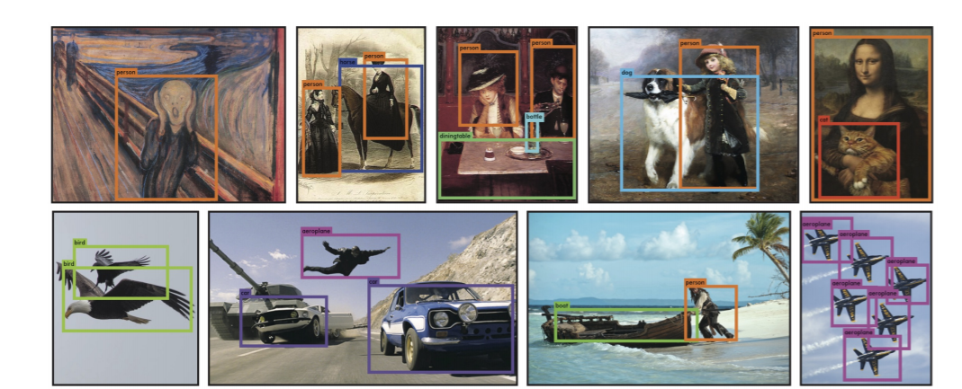
마지막으로, YOLO는 객체의 매우 일반적인 표현을 학습한다.
자연 이미지에서 예술작품과 같은 다른 도메인으로 일반화할 때 DPM 및 R-CNN을 포함한 다른 탐지 방법을 능가한다.
1. Introduction
인간은 이미지를 흘끗 보고, 이미지 안에 어떤 물체가 있는지, 어디에 있는지, 어떻게 상호작용하는지 즉시 알게 된다.
인간의 시각 시스템은 빠르고 정확하여 운전과 같은 복잡한 작업을 거의 의식하지 않고 수행할 수 있다.
물체 감지를 위한 빠르고 정확한 알고리즘을 통해 컴퓨터는 특수 센서 없이 자동차를 운전할 수 있고 보조 장치가 인간 사용자에게 실시간 장면 정보를 전달할 수 있으며 범용 반응형 로봇 시스템의 가능성을 열 수 있다.
현재 탐지 시스템은 분류기의 용도를 변경하여 탐지를 수행한다.
object를 탐지하기 위해 이러한 시스템은 해당 object에 대한 분류기를 가져와서 테스트 이미지의 다양한 위치와 척도에서 해당 object를 평가한다.
deformable parts models (DPM)과 같은 시스템에서는 분류기가 전체 이미지에 걸쳐 일정한 간격으로 실행되는 sliding window 접근 방식을 사용합니다.
R-CNN과 같은 보다 최근의 접근 방식은 region proposal methods 을 사용하여 먼저 이미지에서 potential bounding boxes 를 생성한 다음 이러한 제안된 상자에서 classifier를 실행한다. (2-stage)
분류 후 post-processing 는 bounding boxes 를 세분화하고 중복 탐지를 제거하며 장면의 다른 개체를 기반으로 상자를 다시 찾는 데 사용됩니다
이런 복잡한 pipeline은 각 개별 구성요소가 별도로 훈련되어야 하기 때문에 속도가 느리고 최적화하기 어렵다.
우리는 object detection 를 이미지 픽셀에서 경계 상자 좌표 및 클래스 확률에 이르기까지 단일 회귀 문제로재구성한다. 이 YOLO system을 사용하면 이미지를 한 번만(YOLO) 보고 어떤 개체가 있는지, 어디에 있는지 예측할 수 있다.
YOLO 는 매우 간단하다. Figure 1 참조
Figure 1: The YOLO Detection System. Processing images with YOLO is simple and straightforward. Our system (1) resizes the input image to 448 × 448, (2) runs a single convolutional network on the image, and (3) thresholds the resulting detections by the model’s confidence.
Figure 1: The YOLO Detection System. Processing images with YOLO is simple and straightforward. Our system
(1) resizes the input image to 448 × 448,
(2) runs a single convolutional network on the image
(3) thresholds the resulting detections by the model’s confidence.
A single convolutional network 는 해당 상자에 대한 여러 경계 상자와 클래스 확률을 동시에 예측한다. (1-stage)
YOLO는 전체 영상에 대해 훈련하고 탐지 성능을 직접 최적화한다.
이 통합 모델은 기존의 객체 감지 방법보다 몇 가지 이점이 있다.
첫째, YOLO는 매우 빠르다.
탐지를 회귀 문제로 간주하기 때문에 복잡한 파이프라인이 필요하지 않는다.
우리는 detection을 예측하는데 test 단계에서 새로운 이미지를 Yolo neural network에 넣어주기만 하면 간단하게 실행할 수 있다.
YOLO의 base network는 Titan X GPU에서 배치 처리 없이 초당 45프레임으로 실행되며 빠른 버전은 150fps 이상에서 처리한다.이 방식으로 우리는 video 를 실시간으로 할 수 있다는 것이다. 지연 시간이 25 milliseconds 미만이다. 또한 YOLO는 다른 실시간 시스템의 mAP의 2배 이상을 달성한다.
둘째, YOLO는 예측을 할 때 이미지에 대해 globally으로 추론한다. sliding window 및 d region proposal-based techniques과 달리, YOLO는 훈련 및 테스트 시간 동안 전체 이미지를 보기 때문에 클래스와 그 외관에 대한 상황 정보를 암시적으로 인코딩한다.
Fast R-CNN a top detection method 는 더 큰 컨텍스트를 볼 수 없기 때문에 이미지의 백그라운드 patches를 object로 착각한다.
YOLO는 Fast R-CNN에 비해 백그라운드 오류 횟수의 절반에도 미치지 못한다.
셋째, YOLO는 generalizable representations of objects을 학습한다. (일반화)
자연 이미지에 대해 훈련하고 예술작품에 대해 시험했을 때, YOLO는 DPM 및 R-CNN과 같은 상위 탐지 방법을 큰 폭으로 능가한다. YOLO는 매우 일반적이기 때문에 새로운 도메인이나 예기치 않은 입력에 적용될 때 분해될 가능성이 적다.
YOLO는 여전히 sota detection 시스템에 뒤처져 있다. 이미지의 object를 빠르게 식별할 수 있지만 일부 개체, 특히 작은 개체의 위치를 정확하게 지정하기 위해 고군분투하고 있다.
우리는 우리의 실험에서 이러한 트레이드오프를 더 자세히 조사한다.
우리의 모든 교육 및 테스트 코드는 오픈 소스이다. 다양한 사전 교육을 받은 모델도 다운로드할 수 있다.
2. Unified Detection
우리는 물체 탐지의 개별 구성 요소를 single neural network으로 통합한다. 우리 네트워크는 전체 이미지의 기능을 사용하여 각 경계 상자를 예측한다. 또한 모든 클래스의 모든 경계 상자를 동시에 예측한다. 이는 전체 이미지와 이미지의 모든 개체에 대한 네트워크 상의 이유를 의미한다. YOLO 설계는 높은 평균 정밀도를 유지하면서 종단 간 훈련end-to-end training 과 실시간 속도를 가능하게 한다.
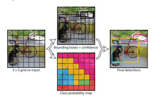
우리 시스템은 입력 이미지를 S × S grid로 나눈다. object 의 중심이 grid cell 로 떨어지면 해당 grid cell이 해당 object를 탐지한다.
각 grid cell 셀은 B 경계 상자와 해당 상자에 대한 신뢰 점수를예측한다.이러한 신뢰도 점수는 상자에 개체가 포함되어 있다는 모형의 신뢰도와 상자가 예측되는 정확도를 반영한다.
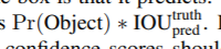
공식적으로 confidence 를 아래와 같이 정희 한다.
해당 cell 에 object 가 없으면 confidence는 0이다.
그렇지 않으면 신뢰 점수가 예측 상자와 실제 실측 사이의 intersection over union (IOU) 과 같기를 원한다.
각 경계 상자는 x, y, w, h, 5개의 예측으로 구성된다. (x, y) 좌표는 그리드 셀의 경계를 기준으로 상자의 중심을 나타낸다.
width and height 는 전체 이미지에 대해 예측된다. 마지막으로 신뢰 예측은 예측 상자와 모든 실제 실측 상자 사이의 IOU를 나타낸다.
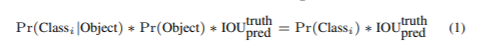
Each grid cell also predicts C conditional class probabilities
이러한 확률은 개체를 포함하는 gird cell에서 조건화된다. 우리는 상자 B의 수에 관계없이 gird cell당 하나의 클래스 확률 집합만 예측한다.
test time 에서 우리는 the conditional class probabilities and the individual box confidence predictions 를 곱한다.
각 상자에 대한 class-specific confidence scores를 제공한다. 이러한 점수는 상자에 해당 클래스가 나타날 확률과 예측 상자가 개체에 얼마나 적합한지 인코딩한다.
Figure 2: The Model. Our system models detection as a regression problem. It divides the image into an S × S grid and for each grid cell predicts B bounding boxes, confidence for those boxes, and C class probabilities. These predictions are encoded as an S × S × (B ∗ 5 + C) tensor.
For evaluating YOLO on PASCAL VOC, we use S = 7, B = 2. PASCAL VOC has 20 labelled classes so C = 20. Our final prediction is a 7 × 7 × 30 tensor.
2.1. Network Design
a convolutional neural network
evevaluate datasetsdetection dataset : PASCAL VOC
fully connected layers 이 output probabilities and coordinates 를 예측하는 동안 network extract features의 initial convolutional layers은 이미지에서 특징을 나타낸다.
우리의 네트워크 아키텍처는 이미지 분류를 위한 GoogleLeNet 모델에서 영감을 받았다.
Our network has 24 convolutional layers followed by 2 fully connected layers.
Instead of the inception modules used by GoogLeNet, we simply use 1 × 1 reduction layers followed by 3 × 3 convolutional layers
The full network is shown in Figure 3.
Figure 3: The Architecture. Our detection network has 24 convolutional layers followed by 2 fully connected layers. Alternating 1 × 1 convolutional layers reduce the features space from preceding layers. We pretrain the convolutional layers on the ImageNet classification task at half the resolution (224 × 224 input image) and then double the resolution for detection.
우리는 또한 fast object detection의 boundaries 를 밀어 넣도록 설계된 빠른 버전의 YOLO를 훈련시킨다.Fast YOLO는 더 적은 컨볼루션 레이어(24개 대신 9개)와 더 적은 필터를 가진 신경망을 사용한다.네트워크의 크기를 제외한 모든 교육 및 테스트 파라미터는 YOLO와 Fast YOLO 간에 동일하다.
network의 최종 output 은 7 × 7 × 30 tensor of predictions.
2.2. Training
우리는 ImageNet 1000 클래스 경쟁 데이터 세트에서 컨볼루션 레이어를 pretrain하였다.
pretraining 을 위해 we use the first 20 convolutional layers from Figure 3 followed by a average-pooling layer and a fully connected layer. 우리는 이 네트워크를 약 일주일 동안 훈련시키고, Cafe's Model Zoo [24]의 GoogleLeNet 모델과 비교할 수 있는 ImageNet 2012 검증 세트에서 88%의 단일 크롭 top-5 정확도를 달성한다 .
우리는 모든 훈련과 추론에 Darknet framework를 사용한다.
그런 다음 모델을 변환하여 탐지를 수행한다. Ren et al. pretrained networks 에 컨볼루션 계층과 연결된 계층을 모두 추가하는 것이 성능을 향상시킬 수 있음을 보여준다. 이들의 예에 따라, 우리는 무작위로 초기화된 가중치를 가진 four convolutional layers and two fully connected layers 를 추가한다. 탐지에는 종종 세분화된 시각적 정보가 필요하므로 네트워크의 입력 해상도를 224 × 224에서 448 × 448로 증가시킨다.
우리의 최종 레이어는 class probabilities and bounding box coordinates 모두 예측한다. We normalize the bounding box width and height by the image width and height so that they fall between 0 and 1. 0 ~ 1 사이로 normalze한다.We parametrize the bounding box x and y coordinates to be offsets of a particular grid cell location so they are also bounded between 0 and 1. 0 ~ 1 사이로 다 한다. w,h , x,y
우리는 최종 계층에 linear activation function를 사용하고 다른 모든 계층은 다음과 같은 leaky rectified linear activation 를 사용한다.
우리는 모델의 출력에서 sum-squared error 를 최적화한다. 우리는 최적화하기 쉽기 때문에 sum-squared error 를 사용하지만 maximizing average precision 한다는 우리의 목표와 완벽하게 일치하지는 않는다. 이것은 localization error를 이상적이지 않을 수 있는 분류 오류와 동등하게 weights를 부여한다.또한 모든 이미지에서 많은 grid cells에는 object가 없다. 이것은 그 cells들의 "confidence" 점수를 0으로 밀어넣고, 종종 물체를 포함하고 있는 cells로부터의 gradient를 압도한다. 이는 모델 불안정성을 초래하여 훈련 초기에 분산될 수 있다.
이를 해결하기 위해 경계 상자 좌표 예측에서 손실을 늘리고 개체를 포함하지 않는 상자에 대한 신뢰 예측에서 손실을 줄인다.
있는것은 5 없는 것은 0.5로 한다.
또한 Sum-squared error 는 large boxes and small boxes의 오차의 가중치를 동일하게 부여한다. 우리의 error metric 은 큰 상자의 작은 편차가 작은 상자보다 덜 중요하다는 것을 반영해야 한다.이를 부분적으로 해결하기 위해 우리는 폭과 높이가 아니라 경계 상자 폭과 높이의 제곱근을 예측한다.
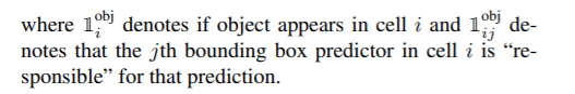
YOLO predicts multiple bounding boxes per grid cell. 여러개의 bouding boxes를 예측한다. 학습 시에는 경계 상자 예측 변수 하나가 각 개체에 대해 책임을 지기를 원한다. 우리는 예측이 실제와 함께 가장 높은 전류 IOU를 갖는 물체를 예측하는 데 "responsible"을 가진 one predictor 을 할당한 between the bounding box predictor에 specialization 로이끈다. Each predictor gets better at predicting certain sizes, aspect ratios, or classes of object, improving overall recall. =>ertain sizes, aspect ratios, or classes of object
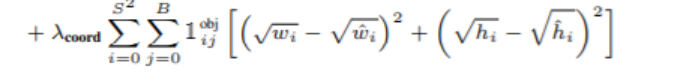
training 중에, 다음과 같은 multi part loss function 를 최적화한다.
Note that the loss function only penalizes classification error if an object is present in that grid cell (hence the conditional class probability discussed earlier). => classification error은 grid cell에 object 있을 경우
It also only penalizes bounding box coordinate error if that predictor is “responsible” for the ground truth box (i.e. has the highest IOU of any predictor in that grid cell). => box predictor 가 ground truth box “responsible” 인경우에만 bounding box coordinate error penalizes
yolov1 loss :
여기서 root를 하는 경우는 작은 물체와 큰 물체가 차이 나기 때문이다.
큰 강아지와 작은 강아지의 loss 차이가 같은 경우에 큰 강아지는 조금만 차이 나는데 작은 강아지 일 경우에는 머리 부분 거의 차이이다. 하지만 loss차이는 같다. => 해결은 root를 해준다. => 작은 object에 대해서 큰 loss를 해준다.
0.5로 곱하는 이유는 :
S = 7 이고 b가 2일 경우에 실제 예측은 7*7*2 = 98개 predict를 한다.
object가 없는 경우가 더 많고 object가 많을 경우 gradient 에 영향을 주어서 0.5를 곱해서 수치를 좀 낮추어서 object 있는 것과 없는 것의 차이를 줄인다.
5를 곱하는 이유는 :
위치를 더 정확하게 할려고 5를 곱한다.
135 epochs
training and validation data sets from PASCAL VOC 2007 and 2012
When testing on 2012 we also include the VOC 2007 test data for training.
batch size 64
momentum 0.9
decay 0.0005
learning rate 은 epoche에 달라 다르게 했다.
높은 학습 속도로 시작하면 불안정한 gradient로 인해 모델이 종종 분리된다.
overfitting을 피하기 위해 dropout and extensive data augmentation
A dropout layer with rate = .5 after the first connected layer prevents co-adaptation between layers.
co-adaptation: 상호적응 문제는,신경망의 학습 중,어느 시점에서 같은 층의 두 개 이상의 노드의 입력 및 출력 연결강도가 같아지면,아무리 학습이 진행되어도 그 노드들은 같은 일을 수행하게 되어 불필요한 중복이 생기는 문제를 말한다.즉 연결강도들이 학습을 통해 업데이트 되더라도 이들은 계속해서 서로 같은 입출력 연결 강도들을 유지하게 되고 이는 결국 하나의 노드로 작동하는 것으로써,이후 어떠한 학습을 통해서도 이들은 다른 값으로 나눠질 수 없고 상호 적응하는 노드들에는 낭비가 발생하는 것이다.결국 이것은 컴퓨팅 파워와 메모리의 낭비로 이어진다.
For data augmentation we introduce random scaling and translations of up to 20% of the original image size
또한 HSV 색 공간에서 이미지의 노출과 포도를 최대 1.5배까지 임의로 조정했다.
색상(Hue), 채도(Saturation), 명도(Value)
2.3. Inference
훈련과 마찬가지로 테스트 이미지에 대한 탐지를 예측하려면 네트워크 평가가 하나만 필요한다.
On PASCAL VOC the network predicts 98 bounding boxes per image and class probabilities for each box. => 98개 bounding box: 7(S) * 7 * 2( B). YOLO는 classifier-based methods과 달리 단일 네트워크 평가만 필요하기 때문에 테스트 시간에 매우 빠르다.
그리드 설계는 경계 상자 예측에서 공간 다양성을 시행한다.object 가 속한 grid cell이 명확하면 네트워크는 각 Object에 대해 하나의 상자만 예측한다. 하지만 , some large objects or objects near the border of multiple cells can be well localized by multiple cells. =>multiple cells 생길 수 있다.=> Non-maximal suppression로 해결할 수 있다. R-CNN 또는 DPM의 경우처럼 성능에 중요하지 않지만, 최대가 아닌 억제 기능은 mAP에서 23%를 추가한다.
2.4. Limitations of YOLO
각 grid cell 은 두 개의 상자만 예측하고 하나의 클래스만 가질 수 있기 때문에 YOLO는 bounding box predictions에 strong spatial constraints을 가한다. 이 spatial constraint은 우리 모델이 예측할 수 있는 가까운 객체의 수를 제한한다. Our model struggles with small objects that appear in groups, such as flocks of birds.=> 작은 물체에 대해서 성능을 올리려고 노력하고 있다.
우리의 모델은 데이터에서 경계 상자를 예측하는 방법을 배우기 때문에, 새로운 또는 특이한 가로 세로 비율이나 구성의 object 로 일반화하기가 어렵다. =>new or unusual aspect ratios or configurations 우리의 모델은 또한 우리의 아키텍처가 입력 이미지에서 여러 down-sampling layer을 가지고 있기 때문에 경계 상자를 예측하는 데 비교적 coarse features 을 사용한다.
마지막으로, detection performance 에 근사한 loss function 에 대해 훈련하는 동안, 우리의 loss function 는 작은 bounding boxes versuslarge bounding boxes 에서 오류를 동일하게 취급한다.큰 상자의 작은 오류는 일반적으로 양호하지만 작은 상자의 작은 오류는 IOU에 훨씬 더 큰 영향을 미친다. Our main source of error is incorrect localization.
3. Comparison to Other Detection Systems
Object detection is a core problem in computer vision. => 핵심문제이다.
Detection pipelines 은 일반적으로 입력 이미지에서 일련의 robust features 하는 것으로 시작한다.
Then, classifiers [36, 21, 13, 10] or localizers [1, 32] are used to identify objects in the feature space.
These classifiers or localizers are run either in sliding window fashion over the whole image or on some subset of regions in the image [35, 15, 39].
We compare the YOLO detection system to several top detection frameworks, 주요 유사점과 차이점을 강조한다.
Deformable parts models. sliding window DPM은 disjoint pipeline을 사용하여 static features을 추출하고 영역을 분류하며 점수가 높은 영역에 대한 경계 상자를 예측한다.우리의 시스템은 본질적으로 다른인 모든 부분을 단일 컨볼루션 신경망으로 교체한다. The network performs feature extraction, bounding box prediction, nonmaximal suppression, and contextual reasoning all concurrently. 네트워크는 static features in-line 기능을 학습하고 탐지 작업에 최적화한다. DPM보다 빠르고 더 정확하다.
R-CNN. R-CNN and its variants은 이미지에서 물체를 찾기 위해 sliding windows 대신 region proposals을 사용한다. Selective Search generates potential bounding boxes, a convolutional network extracts features, an SVM scores the boxes, a linear model adjusts the bounding boxes, and non-max suppression eliminates duplicate detections.이 complex pipeline의 각 단계는 독립적으로 정밀하게 조정되어야 하며 결과 시스템은 매우 느려서 테스트 시간에 영상당 40초 이상 걸린다.
YOLO는 R-CNN과 몇 가지 유사점을 공유한다.각 grid cell은 potential bounding boxes를 제안하고 convolutional features 을 사용하여 해당 상자에 점수를 매긴다. 그러나, 우리의 시스템은 동일한 객체에 대한 여러 탐지를 완화하는 데 도움이 되는 그리드 셀 제안에 spatial constraints을 가한다. 또한 우리 시스템은 선별 검색의 약 2000개보다 이미지당 98개만 훨씬 적은 경계 상자를 제안한다. 마지막으로, 우리의 시스템은 이러한 개별 구성요소를 공동으로 최적화된 단일 모델로 결합한다.
Other Fast Detectors
Deep MultiBox.
OverFeat.
MultiGrasp.
4. Experiments
먼저 YOLO를 PASCAL VOC 2007로 다른 실시간 detection 시스템과 비교한다.
YOLO와 R-CNN variants 의 차이를 이해하기 위해 우리는 YOLO가 만든 VOC 2007과 R-CNN의 최고 성능 버전 중 하나인 Fast R-CNN의 오류를 탐구한다. the different error profiles 을 기반으로 우리는 YOLO를 사용하여 Fast R-CNN 탐지를 다시 검색하고 백그라운드 잘못된 긍정에서 오류를 줄일 수 있다는 것을 보여줌으로써 상당한 효과를 얻을 수 있다.
또한 VOC 2012 결과를 제시하고 mAP를 현재의 sota 방법과 비교한다. 마지막으로 YOLO는 artwork dataset에 대해서도 other detectors 보다 더 좋은 결과로 일반화됨을 보인다.
4.1. Comparison to Other RealTime Systems
Fast YOLO is the fastest object detection method on PASCAL;
Fast R-CNN은 R-CNN의 classification 단계를 빠르게 했지만 selective search
mAP는 높지만 0.5 fps 로 실시간은 아니다.
최근의 Faster R-CNN은 bbox 를 제안하기 위해 selective search 대신 Szegedy 처럼 신경망을 사용한다.
테스트해본 결과 가장 정확한 모델이 7 fps 를 달성하고 덜 정확한 모델은 18 fps 이다. Faster
R-CNN의 VGG16 모델은 mAP 가 10이 더 높은데 YOLO보다 6배 느리다.
Faster R-CNN의 ZeilerFergus 모델은 YOLO보다 2.5 배만 느리지만 덜 정확하다.
4.2. VOC 2007 Error Analysis
YOLO와 다른 sota detector와 차이를 더 상세하게 조사하기 위해 VOC 2007 결과를 상세히 분석해본다.Fast R-CNN은 PASCAL에서 가장 성능이 뛰어난 검출기 중 하나이며 탐지를 공개적으로 사용할 수 있기 때문에 우리는 YOLO를 Fast RCNN과 비교한다.
우리는 Hoiem 등의 방법론과 도구를 사용한다.테스트 시 각 범주에 대해 해당 범주의 상위 N개 예측을 살펴분다. 각 예측은 정확하거나 오차 유형을 기준으로 분류된다.
• Correct: correct class and IOU > .5
• Localization: correct class, .1 < IOU < .5
• Similar: class is similar, IOU > .1
• Other: class is wrong, IOU > .1
• Background: IOU < .1 for any object
Figure 4: Error Analysis: Fast R-CNN vs. YOLO These charts show the percentage of localization and background errors in the top N detections for various categories (N = # objects in that category).
4.3. Combining Fast R-CNN and YOLO
Table 2: Model combination experiments on VOC 2007. We examine the effect of combining various models with the best version of Fast R-CNN. Other versions of Fast R-CNN provide only a small benefit while YOLO provides a significant performance boost.
4.4. VOC 2012 Results
Table 3: PASCAL VOC 2012 Leaderboard. YOLO compared with the full comp4 (outside data allowed) public leaderboard as of November 6th, 2015. Mean average precision and per-class average precision are shown for a variety of detection methods. YOLO is the only real-time detector. Fast R-CNN + YOLO is the forth highest scoring method, with a 2.3% boost over Fast R-CNN.
4.5. Generalizability: Person Detection in Artwork
Figure 5: Generalization results on Picasso and People-Art datasets.
Figure 6: Qualitative Results. YOLO running on sample artwork and natural images from the internet. It is mostly accurate although it does think one person is an airplane.
6. Conclusion
YOLO라는 통합 모델을 도입했는데 구축이 단순하고 학습은 전체 이미지에서 직접 이루어진다. classifier 기반의 방법과 달리 YOLO는 detection 성능에 직접 연관된 손실함수로 학습되고 전체 모델은 결합되어 학습된다.
Fast YOLO는 말그대로 가장 빠른 일반 목적의 사물 detection 시스템이며 YOLO는 최고의 실시간 detection 으로 등극했다. YOLO는 또한 빠르고 강건한 detection 에 의존하는 각종 응용들을 이상적으로 만드는 새로운 영역으로까지 일반화되고 있다.
2. Weakly-Supervised Learning : character level 데이터 만들기
3. region score and the affinity score
Abstract
신경망을 기반으로 한 장면 텍스트 탐지 방법이 최근 등장했고 유망한 결과를 보여준다.
그 전의 학습 방법인 rigid word-level bounding 는 arbitrary shape 텍스트 영역을 나타네는데 학계가 있다.
이 논문에서는 each character and affinity between characters을 탐색하여 텍스트 영역을 효과적으로 탐지하는 새로운 Text Detection 방법을 제안하였다.
개별적인 character level annotations가 적은 것을 극복하기 위하여 우리는 2가지 방법을 제안하였다.
1. 합성 이미지에 대해 주어진 characterlevel annotations
2. 학습된 interm model에 의해 획득된 real image에 대한 추정된 character-level ground-truths
character 사이에 affinity를 추정하기 위해서 , network는 새롭게 제안된 affinity에 대한 representation을 훈련해야 한다.
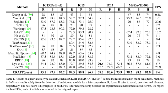
state-of-the-art detectors
결과에 따르면 arbitrarily-oriented, curved, or deformed texts 등에 대해 유연하게 결과를 얻을 수 있다.
1. Introduction
Scene text detection computer vision 에서 많은 관심을 끌고 있다.
예 : instant translation, image retrieval, scene parsing, geo-location, and blind-navigation
위에서 말한 것들은 요즘 deep learning이 발전하면서 좋은 성능을 가지고 있다.
하지만 이런것들은 curved, deformed, or extremely long등에서 single bounding box를 dectect하는데 많은 어려운 케이스가 있다.
character-level awareness는 많은 장점을 가지고 있다. bottom-up 방식으로 연속적인 character를 연결함으로써 많은 장점이 있다. 불행하게도 , 기존의 존재한 text datesets는 characterlevel annotations는 제공하지 않아서 비용이 많이 든다.
이 논문에서 , t localizes the individual character regions and links the detected characters to a text instance. 를 하는 새로운 text detector를 제안하였다.
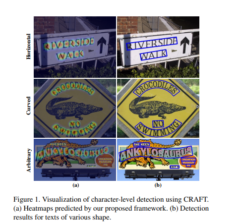
CRAFT for Character Region Awareness For Text detection :
the character region score and affinity score cnn 모델
region score is used to localize individual characters in the image, 이미지에서 개별 character를 localize 하는데 사용
the affinity score is used to group each character into a single instance. 각각의 character를 하나의 instance로 그룹을 해줄 때 사용
bottom-up => MSER [27] or SWT [5]– as a basic component.
deep learningbased text detectors have been proposed by adopting popular object detection/segmentation methods like SSD [20], Faster R-CNN [30], and FCN [23].
Regression-based text detectors:
텍스트 같은 경우 불규칙한 모양을 가지고 있기 때문에 , 이러한 문제를 해결하기 위해 TextBoxes 는 다양한 텍스트 모양을 효과적으로 캐처하기 위해 convolutional kernels and anchor boxes 를 수정했다.
DMPNet quadrilateral sliding windows을 통합하여 문제를 더욱 줄이려고 노력했다.
최근에는 Rotation-Sensitive Regression Detector (RSDD) convolutional filters 를 능동적으로 회전시키면서 회전 불변성 한 feature를 완전히 사용하는 방법이 제안되기도 했다.
However, there is a structural limitation to capturing all possible shapes that exist in the wild when using this approach. 구조적 제한이 있다.
Segmentation-based text detectors
pixel level로 text regions을 찾기 위한 방법론이다.
detect texts by estimating word bounding areas: Multi-scale FCN [7], Holistic-prediction [37], and PixelLink [4]
SSTD는 feature level에서 배경 간섭을 줄임으로써 , text 관련 영역을 향상하는 attention mechanism을 사용하여 regression 과 segmentaition 의 장점을 가질려고 한다.
TextSnake : geometry attributes 특징과 함께 중안 선과 text영역을 예측함으로써 , text 객체를 탐지하는 것을 제안하기도 했다.
End-to-end text detectors
leveraging the recognition result detection and recognition modules simultaneously
FOTS [21] and EAA [10] Mask TextSpotter
It is obvious that training with the recognition module helps the text detector be more robust to text-like background clutters
Character-level text detectors
Zhang et al. [39] MSER [27]
Yao et al.
WordSup [12] : weakly supervised framework to train the characterlevel detector.
Wordsup의 단점은 character representation이 rectangular anchors로 형성된다. 이런한 것은 varying camera viewpoints 각도에 따라서 야기되는 characters의 변형 관점에서 취약하게 된다.
backbone structure 가 제한되여있다. ( SSD )
3. Methodology
우리의 목표는 natural images에서 each individual character 들이 정밀하게 현지화 하는 것이다.
deep neural network a deep neural network to predict character regions and the affinity between characters.
공개 된 character-level dataset 없기 때문에 우리는 weaklysupervised 방식으로 모델을 학습하였다.
3.1. Architecture
backbone : VGG-16
VGG-16 - BN을 사용하였다.
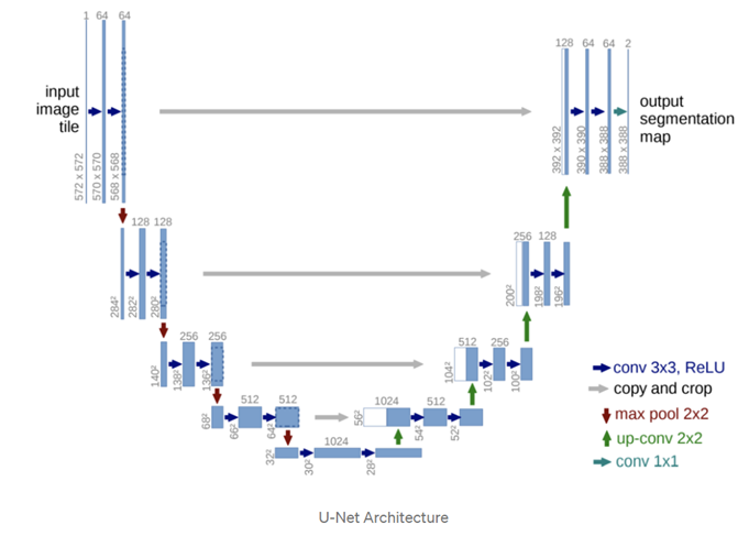
skip connections 이 있고 decoding 부분은 U-netin that it aggregates low-level features과 비슷하다.
U-Net
The final output has two channels as score maps: the region score and the affinity score.
Figure 2. Schematic illustration of our network architecture.
3.2. Training
3.2.1 Ground Truth Label Generation
각 image를 학습 할때 우리는 각 characterlevel bounding boxes region score and the affinity score 의 ground truth label를 생성한다.
•Region score는 해당 픽셀이 문자(Character)의 중심일 확률을 의미.
•Affinity score는 해당 픽셀이 인접한 두 문자의 중심일 확률을 의미.
이 점수를 기반으로 개별 문자가 하나의 단어로 그룹화될 것인지가 결정됨.
•Ground Truth Label 생성
•각 학습 이미지에서 우리는 ground truth label을 character-level bounding boxes로 region score과 affinity score를 생성한다.
•Unlike a binary segmentation map, which labels each pixel discretely, we encode the probability of the character center with a Gaussian heatmap.=> 각 pixel discretely, label을 지정하는 binary segmentation map과 달리 , 우리는 a Gaussian heatmap 을 사용하여 중심의 확률을 인코딩하였다.
•heatmap representation 은 엄격하게 경계가 없는 ground truth regions을 처리 할 경우 높은 유연성을 가진다.
•아래의 이미지는 synthetic image에 대한 라벨 생성 pipeline이다.
•bounding box 내의 각 pixel에 대해 Gaussian distribution value을 직접 구하는 것은 시간이 많이 걸린다.
Figure 3. Illustration of ground truth generation procedure in our framework. We generate ground truth labels from a synthetic image that has character level annotations.
region score and the affinity score:
2차원 isotropic Gaussian map을 준비한다.
이미지 내의 각 문자에 대해 경계상자를 그리고 해당 경계상자에 맞춰 가우시안 맵을 변형시킨다.
변형된 가우시안 맵을 원본 이미지의 경계상자 좌표와 대응되는 위치에 해당하는 Label Map 좌표에 할당한다.
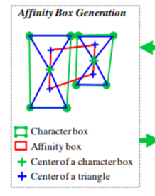
affinity score:
Affinity Score Map은 Region Score Map을 생성할 때 사용했던 Character boxes를 활용한다.
•각 글자의 4개점으로 두개 사각형을 만들 수 있다.
•대각선을 그엇을 때 위 – 아래 삼각형이 생긴다.
•인접한 character box pair 에 대해 , 삼각형 중심점을 이었을 때 만들어지는 사각형이 바로 Affinity box가 된다.
•Region score : Character box 를 label
•Affinity score : Affinity box 를 label
결국 문자 단위(Character-level)의 경계상자(Bounding-Box)만 결정되면 Region Score map과 Affinity Score map을 구할 수 있게된다.
•Figure 3는 box를 바탕으로 라벨을 생성하는 과정이고 , 먼저 2D Gaussian 을 생성하고 , Perspective Transform을 통과하여 , box와 같은 것을 매핑하고 ,마지막으로 해당한 배경을 붙인다.
•결국 문자 단위(Character-level)의 경계상자(Bounding-Box)만 결정되면 Region Score map과 Affinity Score map을 구할 수 있게 된다.
•제안된 Ground-Truth으로정의 된 모델은 receptive fields가 작아도충분히 길거나 큰 텍스트를 감지할 수 있다. 하는 GT 정의는 모델의 receptive fields가 작아도, 크고 긴 텍스트를 검출 가능하게 한다. (이것은 기존의 Bounding Box Regression과 같은 접근 방식이 지닌 문제점을 보완하는 데 탁월한 것으로 보인다.)
•문자 단위 검출은 convolutional filter가 전체 text instance 대신, 문자내및 문자 간의 관계에만 집중할 수 있게 한다.
•문제점:
앞에서 제시된 Ground-Truth를 이미지마다 하나하나 만들기에는 너무 많은 비용이 요구된다.
•기존에 공개되어 있는 대부분의 데이터 집합들은 Annotation이 문자 수준(Character-level)이 아닌 단어 수준(Word-level)으로 annotation이 제공한다.
•이러한 문제를 해결하기 위해 CRAFT 연구팀에서는 기존의 Word-level Annotation이 포함된 데이터 집합을 활용하여 Character-box를 생성하는 방법을 제안했다.
•이 방법에 대해서는 Ground-Truth를 활용한 학습 방법을 살펴본 이후에 소개할 것이다.
3.2.2 Weakly-Supervised Learning
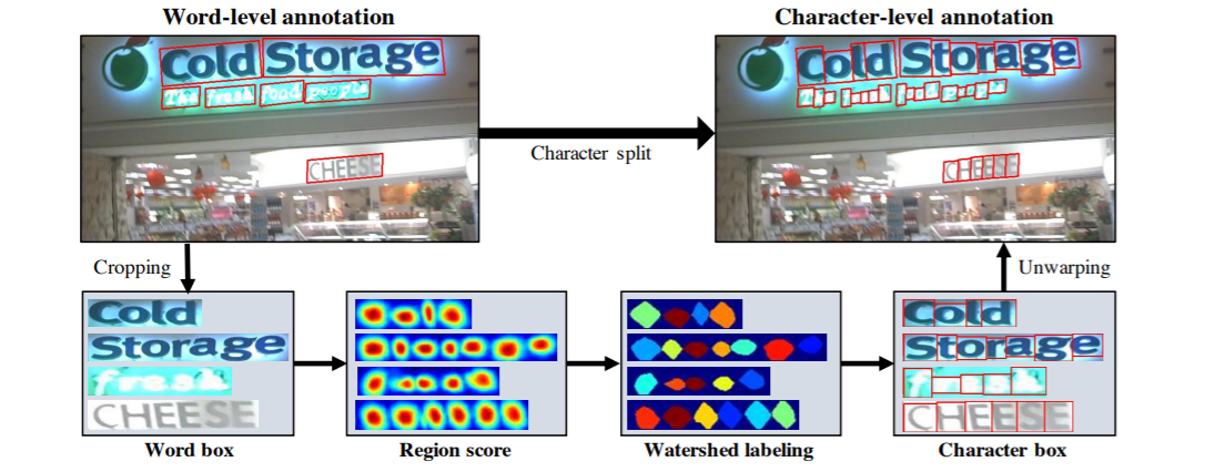
Figure 4. Illustration of the overall training stream for the proposed method. Training is carried out using both real and synthetic images in a weakly-supervised fashion.Figure 6. Character split procedure for achieving character-level annotation from word-level annotation: 1) crop the word-level image; 2) predict the region score; 3) apply the watershed algorithm; 4) get the character bounding boxes; 5) unwarp the character bounding boxes.
•Fig. 6 shows the entire procedure for splitting the characters.(전체 과정)
word-level image는 원본 이미지에서 Cropped 한다.
학습 중인 모델로 crop 된 이미지를 region score를 예측한다.
Watershed algorithm을 이용해 문자 영역을 분리하여 Character box를 결정한다.
마지막으로 분리된 Character box들이 Crop되기 이전의 원본 이미지 좌표로 이동시킨다.
•weak-supervision으로 모델을 학습하면 , 우리는 불완전한 pseudo-GTs 학습할 수 밖에 없다.
•If the model is trained with inaccurate region scores, the output might be blurred within character regions => 정확하지 않은 region scores -> character regions
•이 문제를 방지하기 위해서 논문에서는 텍스트 annotation과 예측한 단어의 길이로 의사 GT의 신뢰도를 평가한다.
pseudo-GTs 신뢰도 평가
•W – training data
•R(w) and l(w) be the bounding box region and the word length of the sample w
•
추정한 단어의 길이
•
샘플에 대한 신뢰도
•
이미지에서 pixel p 위치의 신뢰도.
•픽셀 p에 대해 p가 원본 이미지에서 Word-Box의 영역에 포함된다면 해당 좌표와 대응되는 Confidence Map의 좌표값은Word-Box의 Confidence Score로 설정한다.
•나머지 영역은 모두 1로 설정한다.
중간 모델 학습하기 –Interimmodel
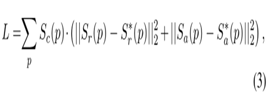
Loss function
•각 pixel에 대한 Region score의 예측값– 정답의 유클리디 거리 오차
•각 pixel에 대한 Affine score의 예측값– 정답의 유클리디 거리 오차
•두 거리 오차의 총합을 Loss로 정의하며 , 이 함수를 최적화 하는 것이 학습의 방향
Confidence map
•이렇게 만든 Confidence map은 Pseudo-GT 데이터 집합을 학습할 때 목적함수(Loss Function) 내에서 사용된다.
Character region score maps
•학습하면서 신뢰도가 점점 높아진다.
•초기 단계에 학습할 경우, 일반 이미지에 익숙하지 않는 텍스트에 대한 region scores가 상대적으로 낮다.
모델 학습할 경우에 신뢰도 점수가 0.5미만일 경우,부정적인 영향을 줄 가능성이 있기 때문에 무시해도 된다. 이런 경우에, individual character 의 Width가 일정하다고 가정하고 단어 영역을 단어 길이로 나누어 character-level 예측한다.
신뢰도는 학습을 위해 0.5로 설정한다.
Figure 5. Character region score maps during training.
3.3. Inference
•추론 단계에서 , 마지막 결과물을 다양하게 할 수 있다.(word boxes or character boxes, and further polygons)
•region score와 affinity score map으로부터 word-level bounding boxes QuadBox를 만드는 방법을 설명한다.
Word-level bounding boxes QuadBox
•post-processing
v이진 맵 MM 을 0으로 초기화
픽셀 p에 대해 Region Score(p) 혹은 Affinity Score(p)가 각각 역치값Tr(p), Ta(p)보다 클 경우 해당 픽셀을 1로 설정
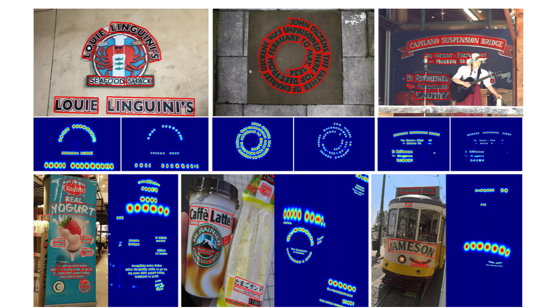
Figure 8. Results on the TotalText dataset. First row: each column shows the input image (top) with its respective region score map (bottom left) and affinity map (bottom right). Second row: each column only shows the input image (left) and its region score map (right).
5. Conclusion
•이 논문에서는 CRAFT라는 문자 단위 텍스트 검출기를 제안했다.
•- 다양한 모양의 텍스트를 상향식으로 검출 가능.
• - 문자에 대한 region score, affinity score를
• - weak-supervision으로 character-level annotation 이 적은 데이터에 대한 학습 방법 제안. interim model을 통해 pseudo-GT 생성
• - 대부분의 공개 데이터셋에 대해 SOTA 성능 달성. fine-tuning 없이 성능을 보여줌으로써 일반화 능력을 입증.
• - 추후 end-to-end model 학습으로 확장.
•큰 이미지에서 비교적 작은 Receptive field로 하나의 문자를 감지하기에 충분하므로, 스케일이 가변적인 텍스트를 검출하는 데 있어서 견고하다.
학습
•Character-level Annotation 데이터 집합의 부족함을 보완하기 위해 2단계의 학습을 수행한다.
1.Ground Truth Label(Region Score와 Affinity Score 생성 Gaussian map )으로 1차 학습 : Interim model 생성
2.Pseudo-Ground Truth Label으로 2차 학습 : Weakly-Supervised Learning
모델을 통해 예측한 Region Score와 Affinity Score를 이용해 최종 결과물을 도출해내는 방법
•2-dimensional isotropic Gaussian map
한계점
•각 문자가 분리되어 있지 않고 연결되는 특정 국가의 언어 혹은 필기체에 대해서는 학습이 쉽지 않다.
•아쉬운 FPS
pseudo라벨:
딥러닝 모델을 훈련시킬때는 다량의 샘플을 지닌 데이터셋이 필수적입니다. 데이터셋에는 보통 이미지들과 그에 맞는 라벨(label, 레이블로 읽어도 됨)들이 들어가 있습니다. 이미지는 비교적 쉽게 얻을 수 있지만, 라벨을 매기는 것은 상당한 시간과 노력을 요구하는 일입니다. 만약이미지 분류(image classification)과제라면, 이미지를 보고 그 이미지의 라벨이 무엇인지 일일이 매겨줘야 합니다. 코끼리 이미지면 코끼리라고, 기린 이미지면 기린이라고, 원숭이 이미지면 원숭이라고 라벨링해줘야 합니다. 상당한 노동력을 요구로 하는 일이죠. 따라서 내가 직접하려면 시간을 많이 써야하고, 남에게 맡기려면 돈을 많이 써야합니다.
그런데 만약 이미지 분류 모델의 성능이 매우 좋다면,top-1 에러가 1%보다 작다면, 그 모델을 통해 예측된 라벨값을 라벨로 사용해도 되지 않을까요? 완벽하게 정확하진 않겠지만, 대부분의 경우에는 맞을 것입니다. 이렇게 생성된 라벨을 의사(pseudo) 라벨로 부를 수 있습니다. 일종의 짝퉁 라벨인 것이죠. 의사 라벨에 너무 의존한다면 너무 위험할 수 있겠지만, 모델 가중치의 pre-training 과정에 사용하는 것은 충분히 가능하다고 봅니다. 실제로 의사 라벨을 이용해서 모델을 훈련시키는 것을 최근 논문들에서 종종 발견하곤 합니다[1].
Large Convolutional Network models 은 ImageNet benchmark(AlexNet) classification에서 상당히 인상적인 성능을 주었다. 하지만 그것들은 왜 성능이 좋은지 왜 향상이 되였는지에 대한 명확한 이해가 없습니다. => 이 이유에 대해 논문에서 재기한다.
intermediate feature layer 과 operation of the classifier의 통찰력을 제공하는 새로운 시각화 기법을 소계하였다.
diagnostic role에 사용되는 이러한 시각화를 통해 ImageNet Classification benchmark AlexNe보다 성능이 뛰어난 모델 아키텍츠를 찾을수 있다.
또한 다른 모델 계층에서 성능 기여를 발견하기 위해 ablation study를 수행한다.
데이터 세트에 대해 일반화 잘됨
softmax classifier is retrained하면 Caltech-101 및 Caltech-256sota
ablation study :의학이나 심리학 연구에서, Ablation Study는 장기, 조직, 혹은 살아있는 유기체의 어떤 부분을 수술적인 제거 후에 이것이 없을때 해당 유기체의 행동을 관찰하는 것을 통해서 장기, 조직, 혹은 살아있는 유기체의 어떤 부분의 역할이나 기능을 실험해보는 방법을 말한다. 이 방법은, experimental ablation이라고도 알려져 있는데, 프랑스의 생리학자 Maria Jean Pierre Flourens이 19세기 초에 개척했다. Flourens은 동물들에게 뇌 제거 수술을 시행하여 신경계의 다른 부분을 제거하고 그들의 행동에 미치는 영향을 관찰했다. 이러한 방법은 다양한 학문에서 사용되어왔으며, 의학이나 심리학, 신경과학의 연구에서 가장 두드러지게 사용되었다.
Machine learning에서, ablation study는 "machine learning system의 building blocks을 제거해서 전체 성능에 미치는 효과에 대한 insight를 얻기 위한 과학적 실험"으로 정의할 수 있다.
Convolution Networks(convnets) : hand-written digit classification and face detection에 우수한 성능을 보여주었다.
visual classification tasks 에서도 탁월한 성능을 제공한다.
주목말한 것은 2012년 ImageNet 2012 classification benchmark, with their convnet model achieving an error rate of 16.4%, compared to the 2nd place result of 26.1%.
convnet 모델에 대한 이러한 새로운 관심에 대한 몇 가지 요인은 다음과 같습니다.
(i) the availability of much larger training sets, with millions of labeled examples;
(ii) powerful GPU implementations, making the training of very large models practical and
(iii) better model regularization strategies, such as Dropout (Hinton et al., 2012).
visualization technique
diagnose potential problems with the model => observe
multi-layered Deconvolutional Network (deconvnet)
1.1. Related Work
네트워크에 대한 직관을 얻기 위해 기능을 시각화하는 것은 일반적인 관행이지만 대부분 픽셀 공간에 대한 투영이 가능한 첫 번째 레이어로 제한됩니다. 상위 계층에서는 그렇지 않으며 활동을 해석하는 방법이 제한적입니다.
문제는 더 높은 계층의 경우 불변성이 매우 복잡하여 간단한 2차 근사로 제대로 캡처되지 않는다는 것입니다.
top-down projections
2. Approach
standard fully supervised convnet models
2.1. Visualization with a Deconvnet
Then we successively (i) unpool, (ii) rectify and (iii) filter to reconstruct the activity in the layer beneath that gave rise to the chosen activation.
Unpooling :
convnet에서 the max pooling operation 는 non-invertible 이지만 , 우리는 switch variables set의 각 pooling region내에서 maxima 의 위치를 기록하여 대략적인 역함수를 얻을 수 있다.
Rectification : relu non-linearities
relu 는 max(0, x) 이여서 기능 맵이 항상 양수임을 보장한다.
Filtering: deconvnet
flipping each filter vertically and horizontally
3. Training Details
One difference is that the sparse connections used in Krizhevsky’s layers 3,4,5 (due to the model being split across 2 GPUs) are replaced with dense connections in our model.
sparse connections-> dense connections
4. Convnet Visualization
Feature Visualization:
Feature Evolution during Training:
The lower layers of the model can be seen to converge within a few epochs. However, the upper layers only develop develop after a considerable number of epochs (40-50), demonstrating the need to let the models train until fully converged.
Feature Invariance:
4.1. Architecture Selection
4.2. Occlusion Sensitivity
4.3. Correspondence Analysis
5. Experiments
5.1. ImageNet 2012
Varying ImageNet Model Sizes:
5.2. Feature Generalization
Caltech-101:
Caltech-256:
PASCAL 2012:
5.3. Feature Analysis
6. Discussion
First, we presented a novel way to visualize the activity within the model.
We also showed how these visualization can be used to debug problems with the model to obtain better results, for example improving on Krizhevsky et al. ’s (Krizhevsky et al., 2012) impressive ImageNet 2012 result.
then demonstrated through a series of occlusion experiments that the model, while trained for classification, is highly sensitive to local structure in the image and is not just using broad scene context.
Finally, we showed how the ImageNet trained model can generalize well to other datasets.
[논문]:Gradient-Based Learning Applied to Document Recognition
LeNet5
LeNet5 간단하게 요약 :
모델 구조
Convolutional Neural Network
subsmapling
우편번호와 필기체 인식하기 위한
XI. Conclusions
학습
CNN을 통해 직접 특징 추출하는 것을 할 필요 없게 되었음.
GTN을 통해 파라메터 튜닝, 레이블링, 경험에 의존한 방법들의 사용을 줄일 수 있었음.
학습할 데이터가 많아지고 , 컴퓨터도 빨라졌다.
그래서 학습이 중요하다.
bACK-propagation algorithm
multi-ayer neural networks
gradient-based learning for Graph transformer Netorks
Maximum Likelihood Principle
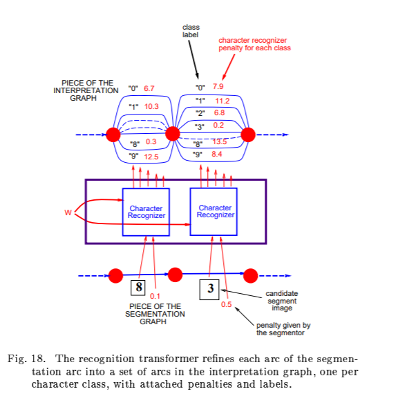
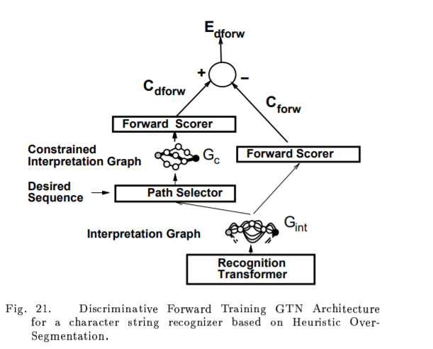
해당 GTN은 전체적인 성능 향상을 위해 여러 모듈들에 대해 Gradient 기반 학습을 하도록 합니다. GTN에 대해 대략적으로 읽어본 결과, 수표 인식을 위해 캐릭터 하나 하나를 분할하기 위한 방법에 대해 설명하는 내용이었습니다
1. Feature extration 전통저긍로 fixed transform
2. segmentation and recognition of objects in image cannot be compeletely decoupled.
3. Hand truthing images to obtain segmented characters for training a character recognizer is expensive and does not take into account the way in which a whole document or sequence of characters will be recognized.
4. Ambiguities inherent in the segmentation, character recognition, and linguistic model should be integrated optimally.
5. traditional recognition systems rely on many hand-crafted heuristics to isolate individually recognizable objects.
이 논문은 다양한 방법으로 handwriten character recognition 를 지원하고 표준화 손글때 digit recognition 을 비교하는 작업이다.
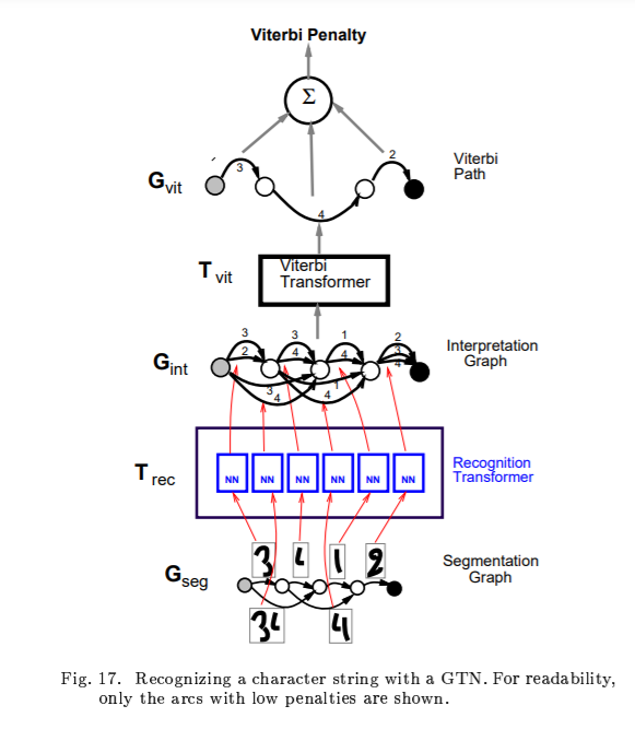
Graph Transformer Networks:
주요한 역할은 original image에서 아직 연결되지 않는 노드들의 유용한 연결을 식별한다.
Two systems for on-line handwriting recognition
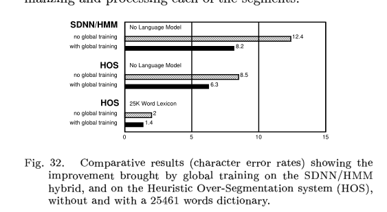
experiments demonstrate global training
GTN: flexibility bankcheck
1. Introduction
pattern recognition systems
이 논문에서의 주오한 메시지는
better pattern recognition systems can be built by relying more on automatic learning, and less on hand-designed heuristics.
End-to-end & Hand-crafted
End-to-end : input original data , output result
Hand-crafted: End-to-end와 대비된다. 사람이 수동으로 설계하여 한 step 마다 step마다 설명이 가능한 것이다.
character recoginition as a case study -> hand-crafted feature extraction
document understanding as a case stuty-> GTN
GTN : that allow training all the modules to optimize a global performance criterion
most pattern recognition systems are built using a combination of automatic learning techniqes and hand-crafted algorithms.
recognizing individual patterns consists in dividing the system into two main moduls
first module, feature extractor, transforms the input patterns so that they can be represented by low-dimensional vectors or short strings of sysmbols
(a) can be easily matched or compared
(b) relatively invariant with respect to transformations and distortions of the input patterns that do not change their nature.
feature extractor : contains most of the prior knowledge and is rather specific to the task. It is also the focus of most of the design effort, because it is often entirely hand-crafted.
classifier , general-purpose and trainable.
1. 특징 추출
Raw input-> Feature vector(특징을 추출한다.)->class scores(거의 변하지 않는다.)
특징 추출이 어렵다.
feature extractors
a combination of three factors have changed this visin over the last decade
1. the availability of low-cost machines with fast arithmetic units allows to rely more on brute-force "numerical" methods than on algorithmic refinements =>계산
2. the availability of large databases for problems with a large market and wide interest, such as handwriting recognition, has enabled designers to rely more on real data and less on hand-crafted feature extraction to build recognition systems => databases
3. 매우 중요한 요인 is the avilability of powerful machine learning techniques that can haldle high-dimensinal inputs and can generate intricate decision functions when fed with these large data sets. => high-dimensional
OCR systems use some form of multi-layer Neural Network trained with back-propagation.
multi-layer neural network
Convolutional Neural Network
LeNet-5 -> this system is in commercial use in the NCR Corporation line of check recognition systems for the baking industry.
Section 소계 :
A. Learning froam Data'
이미지는 크다. pixel로 구성되였다. 수천 만 개 의 weight가 있다.
"numerical" or gradient-based learning
P is the number of training samples,
h is a measure of "effective capacity" or complexity of the machine Statistical Learning
알파 is a number between 0.5 and 1.0 and k is a constant.
h increace Etrain decreases
Etrain줄이는 목적으로 한다.
In practical terms, Structural Risk Minimization is implemented by minimizing
H(W) IS called a regularization fuction
베타 is constant
H(W) is chosen such that it takes large values on parameters W that belong to high-capacity subsets of the parameter space.
minimizingH(W) in effect limits the capacity of the accessible subset of the parameter space,
ghereby controlling the tradeoff between minimizing the training error and minimizing the
expected gap between the training error and test error.
에러를 줄여야 한다.
B. Gradient-Based Learning => loss fuction
Efficient learning algorighms can be devised when the gradient vector can be computed analytically
W is a real-valued vector, with respect to which E(W) is continuous, as well as differentiable almost ererywhere
a popular minimization procedure is the stochastic gradient algorithm -> online updatae
C. Gradient Back-Propagation
the suprising usefulness of such simple gradient descent techniques for complex machine learning tasks was not widely realized unitil the following three events occurred.
1. realization , loss function 은 학습할떄 중요한 원인이 아니다.
2. back-propagation algorighm, to compute the gradient in a non-linear systen compused of several layers of processing.
3. back-propagation procedure applied to multi-layer neural networks with sigmoidal units can solve complicated learning tasks.
기울기 줄이는 것
back-propagation
D. Learning in Real Handuriting Recoginition Systems
Gradient-Based Learning
Convolutional Netwoks
The best neural networks , called Convolutional Networks , are designed to learn to extract relevant features directly from pixel images
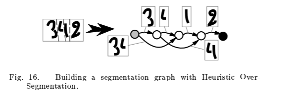
Heuristic over-segmentation:
은닉 마르코프 모형(영어:hidden Markov model,HMM)은 통계적마르코프 모형의 하나로, 시스템이 은닉된 상태와 관찰가능한 결과의 두 가지 요소로 이루어졌다고 보는 모델이다.
training the system at the level of whole strings of characters, rather than at the chracter level
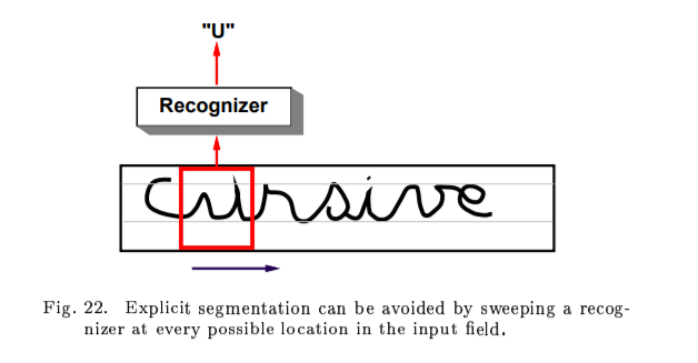
eliminate segmentation altogether
E. Globally Trainable Systems
multiple modules.
Convolutianal Neural Networks for isolated character recognition
a trainable classifier then categorizes the resulting feature vectors into classes.
in this scheme, standard, fully-connected multi-layer networks can be used as classifiers.
1. typical images are large, often with several hundred variables(pixels).
100개 의 hidden units in the first layer, 수많은 weights가 있다.
capacity -> memory
2. a deficiency of fully-connected architectures is that the topology of the input is entirely ignored.
convolutional networks force the extraction of local features by restricting the receptive fields of hidden units to be local
A. Couvolutional Networks
Convolutioanl Networks combine three architectural ideas to ensure some degree of shift, scale, and distortion invariance: 3가지 구조
local receptive fields,
shared weights(or weight replication)
spatial or temporal sub-sampling.
LeNet-5 구조
the input plane receives images of characters that are appoximately size-normalized and centered.
each unit in a layer receives inputs from a set of units located in a small neighborhood in the previous layer.
subsampling: 출력의 일부분만 취하는 것이다.
6 planes
gas 25 uboyts cibbected ti a 5x5
feature map
B. LeNet-5 구조
7 layers (not couting the input)
input 32x32 pixel image
hight-level feature detectors.
Cx: convolutional layers
Sx: subsampling layers
Fx: fully-connected layers
x : layer index.
layer C1 : covolutional layer with 6 feature maps.
Each unit in each feature map is connected to a 5x5 neightborhood in input
The size of the feature map is 28x28 which prevents connection from the input from falling off the boundary
파라미터 156 , 그리고 122,304 개 연결되여있다.
layer S2 sub-sampling layer with 6 feature maps of size 14x14 .
Each unit in each feature map is connected to a 2x2 neighborhood in the corresping feature map in C1.
2x2 receptive fields are non-overlapping
layer C3 : covolutional layer with 16 feature maps.
ach unit in each feature map is connected to a 5x5 neightborhoodS at identiacal locations in a subset of S2's feature maps.
Table1 . shows the set of S2 feature maps conbined by each C3 feature map.
Why not connect every S2 feature map to every C3 feature map?
the reason is twofold.
a non-compelete connection scheme keeps the number of connections within reasonable bounds. 더 중요한것은 이미지의 대칭을 깬다. different feature maps are foreced to extract different(hopefully complementary) features because they get differnt sets of inputs.
the 처음의 6개 feature maps take inputs from every contiguous subsets of three feature maps in S2.
다음의 6개는 take input from every contiguous subset of four
finally the last one takes input from all S2 feature maps.
1,516 trainable parameters and 151,600 connections
layer S4 subsampling layer with 16 feature maps of size 5x5
32 trainable parameters and 2,000 connections
Layer C5 is a convolutional layer with 120 feature maps.
feature map is 1x1
C5 is labeled as a convoluional layer, instead of a fully-connected layer, because if LeNet-5 input were made bigger with everything else kept constant, the feature map dimension would be larger than 1x1.
classical neural networks , units in up to F6 compute a dot product between their input vector and their weight vector, to which a bias is added.
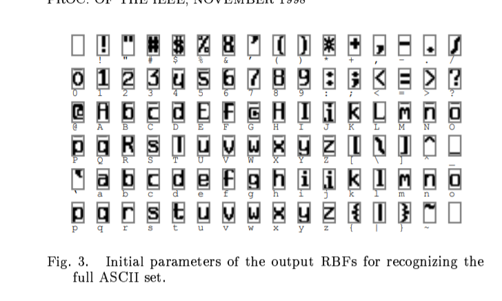
RBF: Radial Basis Function units
그림 초기화 파라미터 -> output RBFs
layer output layer: 10 classes, 0-9 , softmax
C.Loss function
Maximum Likelihood Estimation criterion
Minimum Mean Squared Error(MSE)
Results and Comparison with other methods 결과에 대한 비교
A. database: the modified NIST set -> MNIST
B. Results
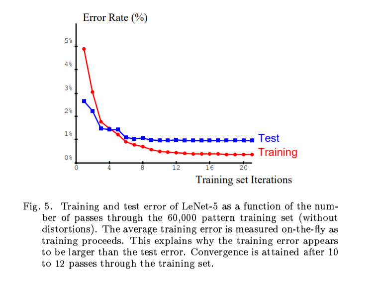
학습 에러가 테스트 에러 보다 크다.
transformations: horizontal and vertical translations, scaling, squeezing(simultaneous horizontal compression and vertical elonggation, or the reverse) and horizontal shearing.
비뚤어진 패턴으로 학습을 하였다. 정확도가 떨어진다. 0.95% -> 0.8%
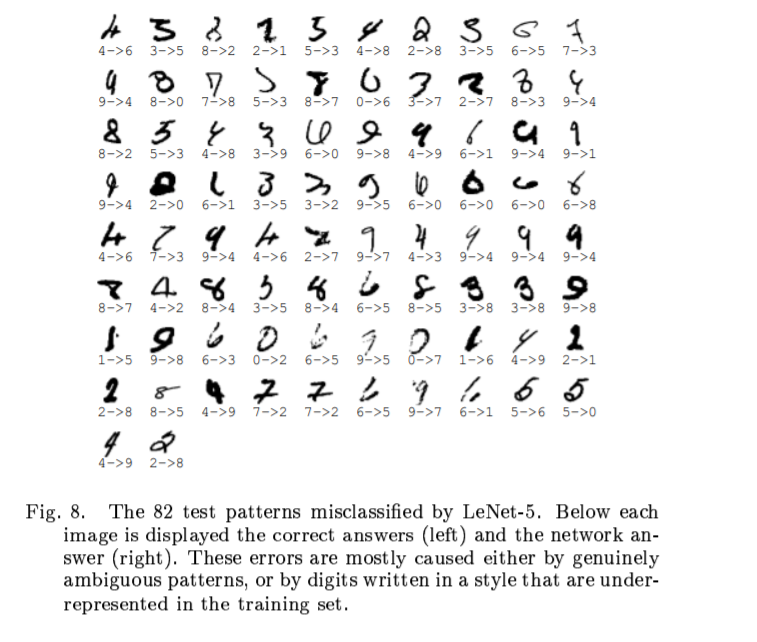
misclassified test examples
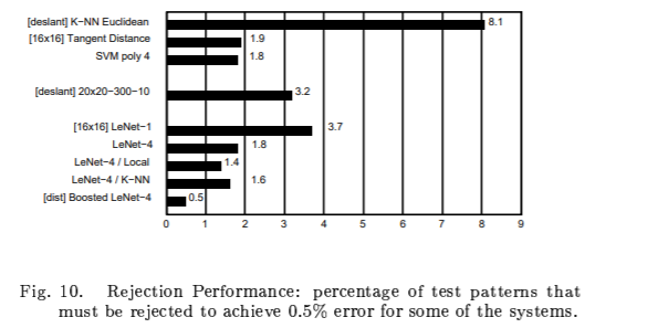
C. Comparison with Other Classifiers
C.1 Linear Classifier, and Pairwise Linear Classifier
Linear Classifier 선형 분류 : Each input pixel value contributes to a weighted sum for each output unit.
The output unit with the hightest sum(including the contribution of a bias constant)
error rate is 12% 8.4% 7.6%
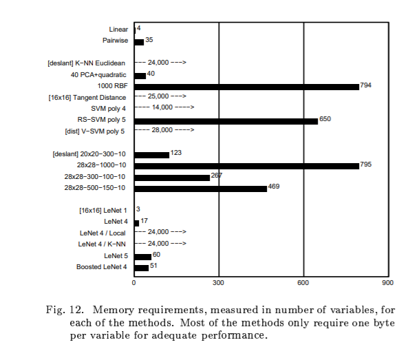
C.2 Baseline Nearest Neighbor Classifier
K-nearest neighbor classifier
메모리가 많이 필요하다.
Euclidean distance
C.3 Pricinpal Component Analysis(PCA) and Polynomial Classifier
Selective Context ATtentional Text Recognizer (SCATTER)
SCATTER는 학습 과정에서 intermediate supervision 기능이있는 스택 형 블록 아키텍처를 사용하여 심층 BiLSTM 인코더의 성공적인 학습을 위한 길을 열어 상황에 맞는 코딩을 개선합니다. 디코딩은 2 단계주의 메커니즘을 사용하여 수행됩니다.
첫 번째 attention step는 CNN backbone의 시각적 특징과 BiLSTM 계층에서 계산 한 컨텍스트 특징에 가중치를 부여하는 것입니다.
두 번째 attention step은 이러한 기능을 시퀀스로 간주하고 시퀀스 간의 관계에 추가합니다.
1. Introduction
recognizing scene text can be divided into two main tasks - text detection and text recognition.
Text detection is the task of identifying the regions in a natural image, that contain arbitrary shapes of text. =>지역 실별
Text recognition deals with the task of decoding a cropped image that contains one or more words into a digital string of its contents. =>cropped image 문자 숫자 등 decoding
text images:
irregular text 임의의 shaped text Fig.1
regular text text with nearly horizontally aligned characters (examples are provided in the supplementary material)
Figure 1: The proposed SCATTER training and inference architecture. We introduce intermediate supervision combined with selective-decoding to stabilize the training of a deep BiLSTM encoder (The circle represents where a loss function is applied). Decoding is done using a selective-decoder that operates on visual features from the CNN backbone and contextual features from the BiLSTM encoder, while employing a two-step attention.
전통적인 text recognition methods [37, 38, 42] detect and recognize text character by character, =>고유한 한계가 있다. sequential modeling and contextual dependencies between characters 활용하지 못한다.
[37] Kai Wang, Boris Babenko, and Serge Belongie. Endto-end scene text recognition. In 2011 International Conference on Computer Vision, pages 1457–1464. IEEE, 2011.
[38] Kai Wang and Serge Belongie. Word spotting in the wild. In European Conference on Computer Vision, pages 591–604. Springer, 2010.
[42] Cong Yao, Xiang Bai, Baoguang Shi, and Wenyu Liu. Strokelets: A learned multi-scale representation for scene text recognition. In Proceedings of the IEEE Conference on Computer Vision and Pattern Recognition, pages 4042–4049, 2014
최신 방법은 STR을 시퀀스 예측 문제로 취급합니다. 우수한 정확도를 달성하는 동안 character-level annotations (per-character bounding box)의 기술을 완화할 필요가 있다
sequence-based methods rely on Connectionist Temporal Classification (CTC) [31, 7], or attention-based mechanisms [33, 16].
four-step STR framework는 individual components 는 다른 알고리즘 교환가능하게 허용한다. This modular framework, along with its best performing component configuration, is depicted in Fig. 1 (a). In this work, we build upon this framework and extend it.
정상적인 scene text를 정확하게 인식하면서 해결되지 않은 문제, 다음과 같은 최근 불규칙한 STR 벤치 마크 ICD15 (SVTP)는 텍스트를 임의의 모양으로 인식하는 문제로 연구 초점을 전환했습니다. Sheng et al. [30]은 다음 개체에 대해 Transformer [35] 모델을 채택했습니다. STR은 변환기 기능을 사용하여 장기적인 컨텍스트 종속성을 캡처합니다. The authors in [16] passed the visual features from the CNN backbone through a 2D attention module down to their decoder. Mask TextSpotter [17]는 탐지 및 인식 작업을 수행합니다. 공유 백본 아키텍처. 인식 단계에서 두 가지 유형의 예측 분기가 사용되며,보다 특정 분기의 출력을 기반으로 최종 예측이 선택됩니다.
The first branch uses semantic segmentation of characters, and requires additional character-level annotations.
The second branch employs a 2D spatial attentiondecoder.
Most of the aforementioned STR methods perform a sequential modeling step using a recursive neural network (RNN) or other sequential modeling layers (e.g., multihead attention [30]), usually in the encoder and/or the decoder. This step is performed to convert the visual feature map into a contextual feature map, which better captures long-term dependencies. In this work, we propose using a stacked block architecture for repeated feature processing, a concept similar to that used in other computer-vision tasks such as in [40] and later in [27, 26]. The authors above showed that repeated processing used in conjunction with intermediate supervision could be used to increasingly refine predictions. In this paper.
visual feature map -> contextual feature map
stacked block architecture
Our method, as depicted in Fig. 1, utilize a stacked block architecture for repetitive processing with intermediate supervision in training, and a novel selective-decoder.
selective-decoder 는 두가지 다른 layers of the network를 수렴한다.
visual features from a CNN backbone
contextual features computed by a BiLSTM layer
이 사이에 two-step 1D attetion mechanism을 사용한다.
Figure 2: Average test accuracy (IIT5K, SVT, IC03, IC13,IC15, SVTP, CUTE) at intermediate decoding steps, compared across different network depths used in training. Given a computation budget, improved results can be obtained by first training a deeper network, and then running only the first decoder(s) during inference.
Figure 2 shows the accuracy levels computed at the intermediate auxiliary decoders, for different stacking arrangements, thus demonstrating the increase in performance as additional blocks are added in succession. block 수에 따라 정확도가 다르다. Interestingly, training with additional blocks in sequence leads to an improvement in the accuracy of the intermediate decoders as well (compared to training with a shallower stacking arrangement).
두가지 공헌이 있다.
1. We propose a repetitive processing architecture for text recognition, trained with intermediate selective decoders as supervision. Using this architecture we train a deep BiLSTM encoder, leading to SOTA results on irregular text. => irregular text.에서 SOTA
2. A selective attention decoder, that simultaneously decodes both visual and contextual features by employing a two-step attention mechanism. The first attention step figures out which visual and contextual features to attend to. The second step treats the features as a sequence and attends the intra-sequence relations. =>두가지 STEP attention mechanism
2. Related Work
3. Methodology
Figure 3: The proposed SCATTER architecture introduces, context refinement, intermediate supervision (additional decoders), and a novel selective-decoder.
3. Methodology
4가지 주요한 componets로 구성되여있다.
1. Transformation: the input text image is normalized using a Spatial Transformer Network (STN) [13]. =>stn을 사용하여 정규화
2. Feature Extraction: maps the input image to a feature map representation while using a text attention module [7]. => text attention module 사용하여 feature map으로
텍스트주의 모델을 사용하여 입력 이미지를 특징 표현에 매핑
3. Visual Feature Refinement: provides direct supervision for each column in the visual features. This part refines the representation in each of the feature columns, by classifying them into individual symbols.=>시각적 기능의 각 열을 직접 모니터링합니다. 특성 열을 별도의 기호로 분류하여 각 특성 열의 표현을 구체화합니다.
4. Selective-Contextual Refinement Block: Each block consists of a two-layer BiLSTM encoder that outputs contextual features. The contextual features are concatenated to the visual features computed by the CNN backbone. This concatenated feature map is then fed into the selective-decoder, which employs a two-step 1D attention mechanism, as illustrated in Fig. 4.각 블록에는 2 계층 BILSTM 인코더 출력 컨텍스트 기능이 포함되어 있습니다. 상황 별 기능과 시각적 기능을 선택적 디코더의 입력으로 결합 (two-step 1D attention mechanism)
Figure 4: Architecture of the Two-Step Attention SelectiveDecoder.
3.1. Transformation
정규화
3.2. Feature Extraction
We use a 29-layer ResNet as the CNN’s backbone, as used in [5]. The output of the feature encoder is 512 channels by N columns.
ResNet으로 이미지 feature map 추출 F = [f1, f2, ..., fN ]. attentional feature map으로 visual feature sequence of length N V = [v1, v2, ..., vN ]
text attention module:기능 필터링, 시맨틱 정보를 사용하여 기능 열을 향상시키고 중복 및 혼동을 억제하며 텍스트 부분에 더 많은주의를 기울입니다.
3.3. Visual Feature Refinement
visual feature sequence V is used for intermediate decoding
This intermediate supervision is aimed at refining the character embedding (representations) in each of the columns of V , and is done using CTC based decoding.
We feed V through a fully connected layer that outputs a sequence H of length N.
The output sequence is fed into a CTC [8] decoder to generate the final output.
loss for this branch, denoted by Lctc , , is the negative log-likelihood of the ground-truth conditional probability, as in [31].
3.4. Selective-Contextual Refinement Block
The features extracted by the CNN 는 각 FIELD에서 제한 되여있으면 , contextual informatoin에 부족하여 고통받고 있다. 이 단점을 완화하기 위하여 we employ a twolayer BiLSTM [9] network over the feature map V , outputting H = [h1, h2, ..., hn]. We concatenate the BiLSTM output with the visual feature map, yielding D = (V, H), a new feature space.
The feature space D is used both for selective decoding, and as an input to the next Selective-Contextual Refinement block.Specifically, the concatenated output of the jth block can be written as Dj = (V, Hj ). The next j + 1 block uses Hj as input to the two-layer BiLSTM, yielding Hj+1, and the j + 1 feature space is updated such that Dj+1 = (V, Hj+1). The visual feature map V does not undergo any further updates in the Selective-Contextual Refinement blocks, however we note that the CNN backbone is updated with back-propagated gradients from all of the selective-decoders. These blocks can be stacked together as many times as needed, according to the task or accuracy levels required, and the final prediction is provided by the decoder from the last block.
3.4.1 Selective-Decoder
two-step attention mechanism 사용
우선 , 우리는 1D self attention 을 사용하여 features D 조작 한다. 완전히 연결된 레이어를 사용하여 지형지 물의주의지도를 계산합니다. 그 다음 , attentional features D '를 얻기 위해 attention map와 D 사이의 곱을 계산합니다. D ' 의 decoding은 attention -decoder 을 분리해서 하기때문에 , t-time-step마다 decode ouputs Yt 가 있다. similar to [5, 2].
3.5. Training Losse
empirically set to 0.1, 1.0 respectively for all j.
3.6. Inference
추론 단계에서는 중간 디코더가 필요하지 않으며 마지막 디코더 만 최종 결과를 출력하는 데 사용됩니다.
4. Experiment
4.1. Dataset
The model is evaluated on four regular scene-text datasets: ICDAR2003, ICDAR2013, IIIT5K, SVT, and
three irregular text datasets: ICDAR2015, SVTP and CUTE
The training dataset is a union of three datasets
MJSynth (MJ) [12]
SynthText (ST) [10]
SynthAdd (SA)) [16]
Regular text
Irregular text
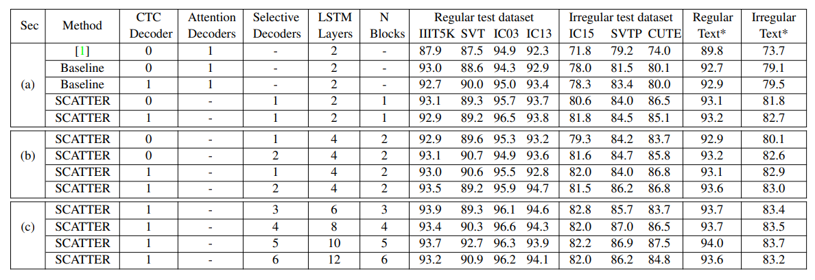
Table 1: Scene text recognition accuracies (%) over seven public benchmark test datasets (number of words in each dataset are shown below the title). No lexicon is used. In each column, the best performing result is shown in bold font, and the second best result is shown with an underline. Average columns are weighted (by size) average results on the regular and irregular datasets. ”*” indicates using both word-level and character-level annotations for training.
4.2. Implementation Details
we use the code of Baek et al.1 [1]
PyTorch the PyTorch2 framework on a Tesla V100 GPU with 16GB memory.
we do not perform any type of pre-training
optimizer : AdaDelta
decay rate 0.95 , gradient clipping with a magnitude 5
batch size of 128 (with a sampling ratio of 40%, 40%, 20% between MJ, ST and SA respectively)
We use data augmentation during training, and augment 40% of the input images, by randomly resizing them and adding extra distortion.
각 Each model is trained for 6 epochs on the unified training set.
validation dataset
image resize : 32 × 100
4.3. Comparison to State-of-the-art
Table 2: Ablation studies by changing the model hyper-parameters. We refer to our re-trained model using the code of Baek et al. 2019 as Baseline. Using intermediate supervision helps to boost results and enables stacking more blocks. Increasing the number of blocks has positive impacts on the recognition performance. * Regular Text and Irregular Text columns are weighted (by size) average results on the regular and irregular datasets respectively
4.4. Computational Costs
Figure 5: Failure cases of our model. GT stands for the groundtruth annotation, and Pred is the predicted result.
5. Ablation Experiments
Throughout this section, we use a weighted-average (by the number of samples) of the results on the regular and irregular test datasets.
Table 3: The table shows example for when repeated processing used in conjunction with intermediate supervision increasingly refines text predictions.Table 4: Performance of each decoder and the oracle. The oracle performance is calculated given the ground truth.
6. Conclusions and Future Work
Supplementary Materials
A. Regular Vs Irregular Text
Figure 6: Examples of regular (IIIT5k, SVT, IC03, IC13) and irregular (IC15, SVTP, CUTE) real-world datasets.
B. Network Pruning - Compute Constraint
C. Examples of Intermediate Predictions
D. Stable Training of a Deep BiLSTM Encoder
Table 5: Average test accuracy at intermediate decoding stages of the network, compared across different training network depths. * Regular Text and Irregular Text columns are weighted (by size) average results on the regular and irregular datasets respectively. Training Blocks N Blocks After Pruning N LSTM Layers After Pruning Regular Text* IrregularTable 6: Examples of intermediate decoders predictions on eight different images, from both regular and irregular text datasets. The presented results in the table, suggests that a selection, voting or ensemble technique could be use to improve results Table 7: The effect of the number of BiLSTM layers used on recognition accuracy. Only by using SCATTER we are able to add BiLSTM layer to improve results. Regular Text and Irregular Text columns are weighted (by size) average results on the regular and irregular datasets. We refer to our re-trained model using the code of Baek et al. 2019 as Baseline.
Image-based sequence recognition은 항상 컴퓨터 비전에서 오랜 연구 주제였습니다. 이 논문에서는 image-based sequence recognition에서 가장 중요하고 어려운 작업 중 하나 인 scene text recognition 문제를 연구합니다. 새로운 신경망 아키텍처는 특징 추출, 시퀀스 모델링 및 변환을위한 통합 프레임 워크를 통합합니다.
feature extraction, sequence modeling and transcription => 통합
이전 scene text recognition 시스템과 비교하여 제안 된 아키텍처에는 다음과 같은 네 가지 속성이 있습니다.
특이점 :
(1) 구성 요소가 개별적으로 학습되고 조정되는 대부분의 기존 알고리즘과 달리 end-to-end 학습 가능합니다.
(2) 임의 길이의 시퀀스를 자연스럽게 처리하고 문자 분할이나 수평 확장 및 정규화를 포함하지 않습니다.(no character segmentation이나 horizontal scale normalization을 포함)
(3) 사전 정의 된 사전에 국한되지 않고 사전 및 사전없이 장면 텍스트 인식 작업에서 놀라운 성능을 달성했습니다.
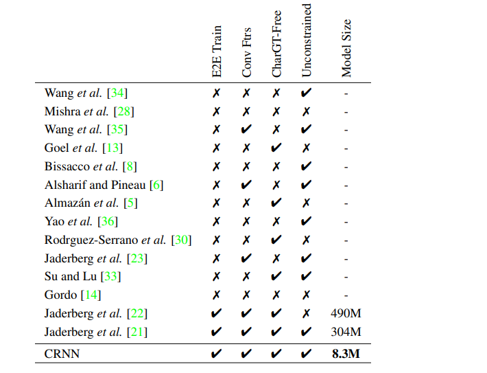
(4) 효과적이고 훨씬 작은 모델을 생성하여 실제 적용 시나리오에 더 실용적입니다.
IIIT-5K, 스트리트 뷰 텍스트 및 ICDAR 데이터 세트를 포함한 표준 벤치 마크에 대한 실험은 제안 된 알고리즘이 기존 기술보다 우월함을 입증했습니다. 또한이 알고리즘은 이미지 기반 점수 인식 작업에서 잘 수행되므로 그 다양성을 분명히 확인할 수 있습니다.
1. Introduction
최근 컨퍼런스는 다양한 시각적 작업에서 심층 신경망 모델, 특히 Deep Convolutional Neural Networks (DCNN)의 대성공에 의해 신경망의 부활을 목격했습니다. 그러나 deep neural networks과 관련된 가장 최근의 연구는 객체 범주의 detection or classification of object categories [12, 25] 에 전념하고 있습니다 . 이 논문에서는 computer vision의 classic problem인 image-based sequence recognition에 중점을 둡니다. 현실 세계에서 안정된 시각적 개체 (예 : 장면 텍스트, 손글씨, 악보)는 분리 된 것이 아니라 시퀀스의 형태로 나타나는 경향이 있습니다. 일반적인 객체 인식과 달리 이러한 객체 시퀀스를 인식하려면 일반적으로 시스템에서 single labels가 아닌 일련의 object labels를 예측해야합니다. 따라서 이러한 객체의 인식은 자연스럽게 시퀀스 인식 문제가 될 수 있습니다. 순차 객체의 또 다른 고유 한 특성은 길이가 크게 달라질 수 있다는 것입니다. 예를 들어 영어 단어 'OK'는 "OK"와 같은 2 자 또는 "“congratulations"와 같은 15 자로 구성 될 수 있습니다. 따라서 DCNN 모델 [25,26]과 같이 가장 많이 사용되는 딥 모델은 시퀀스 예측에 직접 적용 할 수 없습니다. DCNN 모델은 일반적으로 fixed dimensions의 입력 및 출력에서 작동하므로 variable-length label sequence를 생성 할 수 없기 때문입니다. =>DCNN의 단점
object labels: Object labels are the smallest of the museum labels. Their scope is limited to the individual objects they are displayed next to.en.wikipedia.org/wiki/Museum_label
specific sequence-like object (e.g. scene text) 에 대해이 문제를 해결하기위한 몇 가지 시도가있었습니다. 예를 들어 [35, 8]의 알고리즘은 먼저 단일 문자를 감지 한 다음 DCNN 모델을 사용하여 이러한 감지 된 문자를 인식하고 DCNN 모델은 표시된 문자 이미지를 학습에 사용합니다. 이 방법은 일반적으로 원본 문자 이미지에서 각 문자를 정확하게 감지하고 자르기 위해 강력한 문자 감지기를 훈련해야합니다. 일부 다른 방법 (예 : [22])은 scene text recognition 을 이미지 분류 문제로 취급하고 각 영어 단어 (총 90K 단어)에 class label(범주 레이블)을 할당합니다. 훈련 된 모델에는 많은 클래스가 있으며, 이러한 기본 조합이 많고 시퀀스가 100 만 개를 초과 할 수 있기 때문에 중국어 텍스트, 악보 등과 같은 다른 유형의 순차적 객체로 일반화하기 어렵다는 사실이 입증되었습니다. 그렇기 때문에 , DCNN 기반의 현재 시스템은 이미지 기반 시퀀스 인식을 직접 사용할 수 없습니다.
[35] T. Wang, D. J. Wu, A. Coates, and A. Y. Ng. End-to-end text recognition with convolutional neural networks. In ICPR, 2012. 1, 6, 7
[8] A. Bissacco, M. Cummins, Y. Netzer, and H. Neven. Photoocr: Reading text in uncontrolled conditions. In ICCV, 2013. 1, 2, 6, 7
[22] M. Jaderberg, K. Simonyan, A. Vedaldi, and A. Zisserman. Reading text in the wild with convolutional neural networks. IJCV (Accepted), 2015. 1, 2, 3, 6, 7
RNN (Recurrent Neural Network) 모델은 주로 시퀀스를 처리하는 데 사용되는 심층 신경망 family의 또 다른 중요한 branch 입니다.
RNN의 한 가지 장점은 학습 및 테스트 중에 객체 이미지 시퀀스에서 각 요소의 위치가 필요하지 않다는 것입니다. 그러나 입력 객체 이미지를 이미지 특징 시퀀스로 변환하는 전처리 단계는 일반적으로 필수적이다. 예를 들어, Graves et al. [16]은 필기 텍스트에서 기하학적 또는 이미지 특징 세트를 추출하고 Su와 Lu [33]는 단어 이미지를 연속 HOG 특징으로 변환합니다. 전처리 단계는 파이프 라인의 후속 구성 요소와 독립적이므로 RNN을 기반으로하는 기존 시스템은 end-to-end 방식으로 훈련 및 최적화 할 수 없습니다.
[16] A. Graves, M. Liwicki, S. Fernandez, R. Bertolami, H. Bunke, and J. Schmidhuber. A novel connectionist system for unconstrained handwriting recognition. PAMI, 31(5):855–868, 2009. 2
[33] B. Su and S. Lu. Accurate scene text recognition based on recurrent neural network. In ACCV, 2014. 2, 6, 7
신경망을 기반으로하지 않는 몇 가지 전통적인 scene text recognition 방법도이 분야에 인상적인 성능을 가져 왔습니다. 예를 들어, Almazàn et al. [5]와 Rodriguez-Serrano 등 [30]은 단어 이미지와 텍스트 문자열을 공통 벡터 부분 공간에 삽입하고 단어 인식을 검색 문제로 변환하는 것을 제안했습니다. Yao 등 [36]과 Godot 등 [14]은 장면 텍스트 인식을 위해 중간 기능을 사용합니다. 표준 벤치 마크 테스트에서 우수한 성능을 달성했지만 이러한 방법은 일반적으로 이전 신경망 기반 알고리즘보다 성능이 뛰어납니다 [8, 22].
[23] M. Jaderberg, A. Vedaldi, and A. Zisserman. Deep features for text spotting. In ECCV, 2014. 2, 6, 7
[5] J. Almazan, A. Gordo, A. Forn ´ es, and E. Valveny. Word ´ spotting and recognition with embedded attributes. PAMI, 36(12):2552–2566, 2014. 2, 6, 7
[30] J. A. Rodr´ıguez-Serrano, A. Gordo, and F. Perronnin. Label embedding: A frugal baseline for text recognition. IJCV, 113(3):193–207, 2015. 2, 6, 7
[36] C. Yao, X. Bai, B. Shi, and W. Liu. Strokelets: A learned multi-scale representation for scene text recognition. In CVPR, 2014. 2, 6, 7
CRNN = DCNN + RNN
이 논문의 주요 기여는 네트워크 구조가 이미지에서 순차적 인 객체를 식별하는 데 특별히 사용되는 새로운 신경망 모델입니다. 제안 된 신경망 모델은 DCNN과 RNN의 조합이기 때문에 CRNN (Convolutional Recurrent Neural Network)이라고합니다. 순차 이미지의 경우 CRNN은 기존 신경망 모델에 비해 몇 가지 고유 한 장점이 있습니다.
1) detailed annotations (예 : 문자)없이 sequence labels (예 : 단어)에서 직접 학습 할 수 있습니다 .
2) DCNN에는 이미지 데이터에서 직접 정보가 나타내는 동일한 속성을 학습하려면 binarization/segmentation, component localization 지정 등을 포함한 수동 프로세스 기능이나 전처리 단계가 필요하지 않습니다.
3) 동일한 RNN 특성을 가지며 sequence of labels을 생성 할 수 있습니다 .
4) 시퀀스 객체의 길이에 제한을받지 않고 훈련 및 테스트 단계에서만 고도로 정규화하면됩니다 .
5) 기존 기술보다 우수합니다 [23, 8] 장면 텍스트 (텍스트 인식)에서 더 우수하거나 더 경쟁력있는 성능을 얻습니다 .
6) 표준 DCNN 모델보다 훨씬 적은 매개 변수를 포함하고 저장 공간을 덜 차지합니다.
2. The Proposed Network Architecture
그림 1에서 볼 수 있듯이 CRNN의 네트워크 구조는 convolutional layer, recurrent layer, transcription layer의 세 부분으로 구성되어 있습니다.
Figure 1. The network architecture. The architecture consists of three parts: 1) convolutional layers, which extract a feature sequence from the input image; 2) recurrent layers, which predict a label distribution for each frame; 3) transcription layer, which translates the per-frame predictions into the final label sequence.
CRNN의 맨 아래에있는 convolutional layers은 각 input image에서 feature sequence를 자동으로 추출합니다. convolutional network 위에는 convolutional layers이 출력하는 feature sequence의 각 프레임을 예측하기 위해 recurrent network가 설정됩니다. CRNN 상단의 transcription는 recurrent layer의 per-frame 예측을 label sequence로 변환하는 데 사용됩니다. CRNN은 다양한 유형의 네트워크 아키텍처 (예 : CNN 및 RNN)로 구성되어 있지만 loss function를 통해 공동으로 훈련 할 수 있습니다.
2.1. Feature Sequence Extraction
CRNN 모델에서 convolutional layers의 구성 요소는 standard CNN 모델에서 convolutional and max-pooling layers 를 가져 와서 구성됩니다 (fully-connected layers는 제거됨). 이 구성 요소는 입력 이미지에서 순차적 특징 표현을 추출하는 데 사용됩니다. 네트워크에 들어가기 전에 모든 이미지를 동일한 높이로 조정해야합니다. 그런 다음, recurrent layers의 입력 인 convolutional layers 구성 요소에 의해 생성 된 feature maps에서 일련의 feature vectors를 추출합니다. 특히, feature sequence의 각 feature vectors는 feature maps의 열에서 왼쪽에서 오른쪽으로 생성됩니다. 즉, i 번째 feature vector는 모든 맵의 i 번째 열을 연결 한 것입니다. 설정에서 각 열의 너비는 single pixel로 고정됩니다.
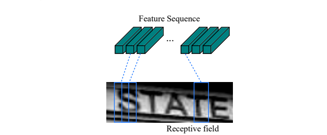
convolution, max-pooling, and elementwise activation function는 local regions에서 작동하므로 translation invariant입니다. 따라서 e feature maps의 각 열은 원본 이미지의 직사각형 영역 (termed the receptive field)에 해당하며, 이러한 직사각형 영역은 왼쪽에서 오른쪽으로 특징 맵의 해당 열과 동일한 순서입니다. 그림 2에서 볼 수 있듯이 특징 시퀀스의 각 벡터는 수용 필드와 연관되어 있으며 영역의 이미지 설명 자로 간주 될 수 있습니다.
Figure 2. The receptive field. Each vector in the extracted feature sequence is associated with a receptive field on the input image, and can be considered as the feature vector of that field.
강력하고 풍부하며 훈련이 가능하기 때문에 다양한 유형의 시각적 인식 작업에서 심층 컨볼 루션 기능이 널리 사용되었습니다 [25,12]. 이전의 일부 방법은 장면 텍스트와 같은 유사한 객체 시퀀스의 강력한 표현을 학습하기 위해 CNN을 채택했습니다 [22]. 그러나 이러한 방법은 일반적으로 CNN을 통해 전체 이미지의 전체 표현을 추출한 다음 로컬 깊이 기능을 수집하여 시퀀스 유사 객체의 각 구성 요소를 식별합니다. CNN은 고정 된 입력 차원을 충족하기 위해 입력 이미지를 고정 된 크기로 조정해야하므로 길이의 큰 변화로 인해 시퀀스와 같은 객체에는 적합하지 않습니다. CRNN에서는 시퀀스와 유사한 객체의 길이가 변경되지 않도록 깊이 특성을 시퀀스 표현에 전달합니다.
2.2. Sequence Labeling
깊은 양방향 순환 신경망은 컨볼 루션 계층 위에 반복 계층으로 구축됩니다. 각 Xt에 대한 순환 계층 티 레이블 Yt 예측 티 , 여기서
, X는 Feature sequence 입니다.
recurrent layers의 장점은 세 가지입니다.
우선, RNN은 sequence내에서 contextual정보를 캡처하는 강력한 기능을 가지고 있습니다. image-based sequence recognition을 사용하는 상황 별 신호는 각 기호를 독립적으로 처리하는 것보다 더 안정적이고 유용합니다. scene text recognition을 예로 들어 넓은 문자를 완전히 설명하려면 여러 연속 프레임이 필요할 수 있습니다 (그림 2 참조). 또한 배경을 관찰 할 때 일부 모호한 문자는 구별하기가 더 쉽습니다. 예를 들어 문자를 개별적으로 인식하는 것보다 높이를 비교하여 "il"을 인식하는 것이 더 쉽습니다.
둘째, RNN은 오류 차이를 입력 즉, 컨볼 루션 계층으로 역 전파 할 수 있으므로 통합 네트워크에서 재생 계층과 컨볼 루션 계층을 공동으로 훈련 할 수 있습니다.
셋째, RNN은 처음부터 끝까지 모든 길이의 시퀀스에서 작동 할 수 있습니다.
Figure 3. (a) The structure of a basic LSTM unit. An LSTM consists of a cell module and three gates, namely the input gate, the output gate and the forget gate. (b) The structure of deep bidirectional LSTM we use in our paper. Combining a forward (left to right) and a backward (right to left) LSTMs results in a bidirectional LSTM. Stacking multiple bidirectional LSTM results in a deep bidirectional LSTM.
전통적인 RNN 유닛은 input and output layers 사이에 self-connected hidden layer를 가지고 있습니다. 프레임 xt가 시퀀스에서 수신 될 때마다 현재 입력 xt와 과거 상태 ht-1을 입력으로 취하는 비선형 함수를 사용하여 내부 상태 ht를 업데이트합니다. 그리고 과거 상태 h t − 1 입력 값 :
. 그런 다음 yt는 ht의 기준으로 만들어졌다 . 이러한 방식으로 과거 컨텍스트가
캡처되고 예측에도 사용됩니다. 그러나 전통적인 RNN 유닛은 vanishing gradient problem [7] 로 인해 저장할 수있는 컨텍스트의 범위를 제한하고 훈련 프로세스의 부담을 증가시킵니다. Long-Short Term Memory [18, 11] (LSTM)은 일종의 RNN 단위로, 특히이 문제를 해결하는 데 사용됩니다. Long-Short Term Memory [18, 11] (LSTM)M (illustrated in Fig. 3) 은 memory cell와 three multiplicative gates, 즉 input, output and forget gates 로 구성됩니다. 개념적으로 메모리 유닛은 과거 컨텍스트를 저장하고 입력 및 출력 게이트를 통해 유닛이 컨텍스트를 오랫동안 저장할 수 있습니다. 동시에 장치의 메모리는 forget gate 를 통해 지울 수 있습니다. LSTM을 사용하면 일반적으로 이미지 기반 시퀀스에서 발생하는 long-range dependencies을 캡처 할 수 있습니다.
LSTM은 방향성이 있으며 과거 컨텍스트 만 사용합니다. 그러나 이미지 기반 시퀀스에서는 양방향의 컨텍스트가 유용하고 서로 보완 적입니다. 따라서 우리는 [17]에 따라 두 개의 LSTM (하나는 앞뒤로)을 bidirectional LSTM으로 결합합니다. 또한 여러 bidirectional LSTM을 스택하여 그림 3.b에 표시된 것처럼 deep bidirectional LSTM을 생성 할 수 있습니다. deep structure는 shallow 구조보다 더 높은 수준의 추상화를 허용하며 음성 인식 작업에서 상당한 성능 향상을 달성했습니다 [17].
순환 계층에서 오류는 BPTT (Back-Propagation Through Time )를 통해 그림 3.b에 표시된 화살표의 반대 방향으로 전파됩니다. rnn의 맨 아래에서 전파 된 오류 시퀀스가 그래프로 연결되고 피쳐 맵을 피쳐 시퀀스로 변환하는 작업이 반전되어 convolutional 계층으로 피드백됩니다. 실제로 컨볼 루션 레이어와 반복 레이어 사이의 다리 역할을하는 "Map-to-Sequence"라는 사용자 지정 네트워크 레이어를 만듭니다.
RNN 장점 -> RNN단점 -> LSTM -> bidirectional LSTM
2.3. Transcription
Transcription은 per-frame RNN 예측을 label sequence로 변환하는 프로세스입니다. Mathematically, 변환은 각 프레임의 예측에 따라 가장 높은 확률을 가진 label sequence를 찾는 것입니다. 실In practice 사전 기반 번역과 사전 기반 전사의 두 가지 변환 모드가 있습니다.lexicon-free and lexicon-based transcriptions . 사전은 맞춤법 검사 사전과 같이 예측이 제한된 태그 시퀀스 세트입니다. 사전 없음 모드에서는 사전없이 예측이 이루어집니다. 사전 기반 모드에서는 확률이 가장 높은 태그 시퀀스를 선택하여 예측합니다.
2.3.1 Probability of label sequence
우리는 Graves 등이 제안한 CTC (Connectionist Temporal Classification) 계층에 정의 된 조건부 확률을 사용합니다 [15].label l 의 각 프레임의 예측 확률은 y = y 1, ..., Y t로 기록되며 특정 위치를 고려하지 않습니다. 따라서이 확률의 negative log-likelihood 을 네트워크 훈련의 대상으로 사용할 때 이미지와 해당 레이블 시퀀스 만 필요하므로 단일 문자의 위치를 표시하는 작업을 피할 수 있습니다.
조건부 확률의 표현은 다음과 같이 간략하게 설명됩니다:
The input is a sequence y = y1, . . . , yT where T is the sequence length.
여기서
는 집합
의 확률 분포이며 , 그중에서 L는ㄴ task중의 전부 lables를 포함하고 있다. (예: english characters) ,예를 들면 "blank"라벨로 표시한다. sequence-to-sequence mapping function B is defined on sequence
where T is the length. B는 먼저 repeated labels 를 삭제 한 다음 "blank"을 삭제하고 π를 l에 매핑합니다. 예를 들어 B는 "–hh-e-l-ll-oo –"( '-‘는 blank’로 표시 )를 "hello"에 매핑합니다. 그런 다음 조건부 확률은 확률의 합으로 정의되고 모든 π는 B에서 l로 매핑됩니다.
직접 계산 Eq. 1은 exponentially large number의 합계 항목으로 인해 계산적으로 실행 불가능합니다. 그러나 Eq. 1은 설명 된 앞으로 뒤로 알고리즘을 사용하여 계산 [15]에서 효율적일으로 계산 할 수 있습니다.
2.3.2 Lexicon-free transcription =>사전이 존재하지 않는lexicon-free 모드에서는 예측은 어떤 lexicon없이 만들어진다.
이 모드에서는 Eq. 1에 정의 된 확률이 가장 높은 시퀀스가 예측으로 사용됩니다. 정확한 해를 찾을 수있는 방법이 없기 때문에 [15]의 전략을 채택합니다. 시퀀스는 근사치에 의해 발견됩니다. 즉, 각 타임 스탬프에서 확률이 가장 큰 레이블이 사용되고 결과 시퀀스가 매핑됩니다.
2.3.3 Lexicon-based transcription => 사전이 존재한다. 시간이 오래 걸린다.
사전이 존재하는 lexicon-based transcriptions 모드에서 예측은 가장 높은 가능성을 가진 라벨 시퀀스의 선택으로 만들어진다.
However, for large lexicons, e.g. the 50k-words Hunspell spell-checking dictionary [1], it would be very time-consuming to perform an exhaustive search over the lexicon, i.e. to compute Equation 1 for all sequences in the lexicon and choose the one with the highest probability. To solve this problem, we observe that the label sequences predicted via lexicon-free transcription, described in 2.3.2, are often close to the ground-truth under the edit distance metric.
사전 기반 모드에서 각 테스트 샘플은 사전과 연관됩니다. 기본적으로 태그 시퀀스는 수학 식 1에 정의 된 조건부 확률이 가장 높은 사전에서 시퀀스를 선택하여 식별한다. 그러나 Hunspell 맞춤법 검사 사전 (예 : 50,000 단어 [1])과 같은 대형 사전의 경우 사전에 대한 철저한 검색, 즉 사전의 모든 시퀀스에 대해 방정식 1을 계산하고 확률이 가장 높은 사전을 선택하는 데는 시간이 많이 걸립니다. 이 문제를 해결하기 위해 우리는 2.3.2에서 설명한 사전없는 전사에 의해 예측 된 태그 시퀀스가 일반적으로 편집 거리 측정에서 실제 결과에 가깝다는 것을 관찰했습니다. 즉, nearest-neighbor candidates로 검색을 제한 할 수 있습니다. 여기서는 최대 편집 거리이며, 사전이없는 모드에서 사전에서 전사 된 시퀀스입니다.
BK-tree data structure [9]
BK 트리 데이터 구조 [9]는 which is a metric tree specifically adapted to discrete metric spaces. BK 트리의 검색 시간 복잡도는 사전 크기입니다. 따라서이 체계는 매우 큰 사전으로 쉽게 확장 할 수 있습니다. 우리의 방법에서 사전은 오프라인으로 BK 트리를 구성합니다. 그런 다음 트리를 사용하여 빠른 온라인 검색을 수행하고 편집 거리보다 작거나 같은 시퀀스를 찾아 시퀀스를 쿼리합니다.
2.4. Network Training
stochastic gradient descent (SGD)
Gradients are calculated by the back-propagation algorithm
In particular, in the transcription layer, error differentials are back-propagated with the forward-backward algorithm, as described in [15].
In the recurrent layers, the Back-Propagation Through Time (BPTT) is applied to calculate the error differentials
Back-Propagation Through Time : 위와 같은 특성들 때문에, RNNs를 학습시키기 위해서는 기존의 단순한 Neural Networks를 학습시키기 위해서 사용하던 Backpropagation 알고리즘과는 조금은 다른 방법이 필요하다. 이를 Backpropagation Through Time(BPTT) 알고리즘이라고 부른다.
optimization : ADADELTA [37] to automatically calculate per-dimension learning rates.
Compared with the conventional momentum [31] method, ADADELTA 에서 수동으로 learning rate 설정할 필요 없다. . More importantly, we find that optimization using ADADELTA converges faster than the momentum method.
3. Experiments
scene text recognition and musical score recognition
The datasets and setting for training and testing are given in Sec. 3.1, =>dataset
the detailed settings of CRNN for scene text images is provided in Sec. 3.2, =>setting CRNN
and the results with the comprehensive comparisons are reported in Sec. 3.3. => 결과를 비교
To further demonstrate the generality of CRNN, we verify the proposed algorithm on a music score recognition task in Sec. 3.4. => music score recognition 에서
제안 된 CRNN 모델의 효과를 평가하기 위해 우리는 scene text recognition and musical score recognition을위한 표준 벤치 마크 데이터 세트에 대한 실험을 수행했습니다. 데이터 세트 및 훈련 테스트 설정은 섹션 3.1에 표시되고 장면 텍스트 이미지의 CRNN 세부 설정은 섹션 3.2에 표시되며 포괄적 인 비교 결과는 섹션 3.3에보고됩니다. CRNN의 일반화를 더욱 입증하기 위해 3.4 절에서 점수 인식 과제에 제안 된 알고리즘을 검증했다.
3.1. Datasets
장면 텍스트 인식에 대한 모든 실험에서 Jaderberg 등 [20]이 발표 한 합성 데이터 세트 (Synth)를 훈련 데이터로 사용합니다. 데이터 세트에는 8 백만 개의 학습 이미지와 해당 실제 단어가 포함됩니다. 이러한 이미지는 합성 텍스트 엔진에 의해 생성되며 매우 사실적입니다. 우리의 네트워크는 합성 데이터에 대해 한 번 훈련되었고 훈련 데이터에 대한 미세 조정없이 다른 모든 실제 테스트 데이터 세트에서 테스트되었습니다. CRNN 모델은 순수 합성 텍스트 데이터에 대해 학습되었지만 표준 텍스트 인식 벤치 마크 데이터 세트의 실제 이미지에서 잘 작동합니다.
장면 텍스트 인식의 성능 평가를위한 4 개의 인기 벤치 마크 데이터 세트, 즉 ICDAR 2003 (IC03), ICDAR 2013 (IC13), IIIT 5k-word (IIIT5k) 및 스트리트 뷰 텍스트 (SVT)가 있습니다.
IC03 [27] 테스트 데이터 세트에는 텍스트 경계 상자가 표시된 251 개의 장면 이미지가 포함되어 있습니다. Wang et al. [34], 우리는 영숫자가 아닌 문자 또는 3 자 미만의 문자를 포함하는 이미지를 무시하고 860 개의 잘린 텍스트 이미지로 테스트 세트를 얻습니다. 각 테스트 이미지는 Wang et al. [34]에 의해 정의 된 50 단어 사전과 연관되어 있습니다. 각 이미지의 모든 단어를 결합하여 완전한 사전을 만드십시오. 또한 Hunspell 맞춤법 검사 사전 [1]의 단어로 구성된 5 만 단어 사전을 사용합니다.
IC13 [24] 테스트 데이터 세트는 IC03의 데이터 대부분을 상속했습니다. 1015 개의 실제 잘린 단어 이미지가 포함되어 있습니다.
IIIT5k [28]에는 인터넷에서 수집 한 3000 개의 잘린 단어 테스트 이미지가 포함되어 있습니다. 각 이미지는 50 단어 사전 및 1000 단어 사전과 연결됩니다.
SVT [34] 테스트 데이터 세트는 Google 스트리트 뷰에서 수집 한 249 개의 스트리트 뷰 이미지로 구성됩니다. 647 개의 단어 이미지가 잘라졌습니다. 각 단어 이미지에는 Wang et al. [34]에 의해 정의 된 50 단어 사전이 있습니다.
3.2. Implementation Details
실험에서 사용한 네트워크 구성은 Table 1.에 요약되어 있습니다. convolutional layers의 아키텍처는 VGG-VeryDeep [32]의 아키텍처를 기반으로합니다. recognizing English texts에 적합하도록 조정되었습니다. 3rd and the 4th maxpooling layers 에서는 기존의 squared 대신 t 1 × 2 sized rectangular pooling windows을 사용합니다. 이 조정은 더 넓은 피쳐 맵을 생성하므로 더 긴 피쳐 시퀀스가 생성됩니다. 예를 들어, 10 개의 문자가 포함 된 이미지는 일반적으로 크기가 100x32이고 여기에서 25 프레임의 특징 시퀀스를 생성 할 수 있습니다. 이 길이는 대부분의 영어 단어의 길이를 초과합니다. 가장 중요한 것은 직사각형 풀 창에서 직사각형 수용 필드 (그림 2 참조)를 생성하여 i 및 l과 같은 좁은 모양의 문자를 인식하는 데 도움이됩니다.
Table 1. Network configuration summary. The first row is the top layer. ‘k’, ‘s’ and ‘p’ stand for kernel size, stride and padding size respectively
네트워크에는 deep convolutional layers뿐만 아니라 recurrent layers도 있습니다. 둘 다 훈련하기 어렵다는 것은 잘 알려져 있습니다. batch normalization [19] 기술은 이러한 심층 네트워크를 훈련하는 데 매우 유용하다는 것을 발견했습니다. 5th and 6th convolutional layers respectively 뒤에 각각 두 개의 batch normalization layers를 삽입합니다. 배batch normalization layers를 사용하는 훈련 프로세스가 크게 가속화됩니다.
사용자 정의 구현 LSTM 유닛 (Torch7 / CUDA), transcription layer (C ++) 및 BK-tree data structure (C ++)를 사용하여 Torch7 [10] 프레임 워크 내에서 네트워크를 구현했습니다. 실험은 2.50GHz Intel (R) Xeon E5-2609 CPU, 64GB RAM 및 NVIDIA (R) Tesla (TM) K40 GPU가있는 워크 스테이션에서 수행되었습니다. =>gpu환경
네트워크는 ADADELTA로 훈련되고 매개 변수 ρ는 0.9로 설정됩니다.
훈련 중에 모든 이미지는 훈련 프로세스의 속도를 높이기 위해 100x32로 조정됩니다.
training process은 수렴에 도달하는 데 약 50 시간이 걸립니다.
Testing images are scaled to have height 32 . 너비는 높이에 비례하여 조정되지만 최소 100 픽셀입니다.
average testing time은 0.16 초 / 샘플이며 IC03에서 측정 된 사전이 없습니다. 대략적인 사전 검색은 IC03의 50k 사전에 적용되고 매개 변수 δ는 3으로 설정됩니다. 각 샘플을 테스트하는 데 평균 0.53 초가 걸립니다.
3.3. Comparative Evaluation
4가지 public datasets, shown in Table 2.
Table 2. Recognition accuracies (%) on four datasets. In the second row, “50”, “1k”, “50k” and “Full” denote the lexicon used, and “None” denotes recognition without a lexicon. (*[22] is not lexicon-free in the strict sense, as its outputs are constrained to a 90k dictionary.
[22] M. Jaderberg, K. Simonyan, A. Vedaldi, and A. Zisserman. Reading text in the wild with convolutional neural networks. IJCV (Accepted), 2015. 1, 2, 3, 6, 7
Unlike [22], CRNN is not limited to recognize a word in a known dictionary, and able to handle random strings (e.g. telephone numbers), sentences or other scripts like Chinese words. Therefore, the results of CRNN are competitive on all the testing datasets.
Table 3. Comparison among various methods. Attributes for comparison include: 1) being end-to-end trainable (E2E Train); 2) using convolutional features that are directly learned from images rather than using hand-crafted ones (Conv Ftrs); 3) requiring no ground truth bounding boxes for characters during training (CharGT-Free); 4) not confined to a pre-defined dictionary (Unconstrained); 5) the model size (if an end-to-end trainable model is used), measured by the number of model parameters (Model Size, M stands for millions).
E2E Train: This column is to show whether a certain text reading model is end-to-end trainable, without any preprocess or through several separated steps, which indicates such approaches are elegant and clean for training. As can be observed from Table 3, only the models based on deep neural networks including [22, 21] as well as CRNN have this property.
Conv Ftrs: This column is to indicate whether an approach uses the convolutional features learned from training images directly or handcraft features as the basic representations.
CharGT-Free: This column is to indicate whether the character-level annotations are essential for training the model. As the input and output labels of CRNN can be a sequence, character-level annotations are not necessary. Unconstrained: This column is to indicate whether the trained model is constrained to a specific dictionary, unable to handling out-of-dictionary words or random sequences.Notice that though the recent models learned by label embedding [5, 14] and incremental learning [22] achieved highly competitive performance, they are constrained to a specific dictionary
3.4. Musical Score Recognition
Figure 4. Blue line graph: recognition accuracy as a function parameter δ. Red bars: lexicon search time per sample. Tested on the IC03 dataset with the 50k lexicon.
Optical Music Recognition (OMR)
Figure 5. (a) Clean musical scores images collected from [2] (b) Synthesized musical score images. (c) Real-world score images taken with a mobile phone camera.Table 4. Comparison of pitch recognition accuracies, among CRNN and two commercial OMR systems, on the three datasets we have collected. Performances are evaluated by fragment accuracies and average edit distance (“fragment accuracy/average edit distance”).
For testing, we create three datasets:
1) “Clean”,which contains 260 images collected from [2]. Examples are shown in Fig. 5.a;
2) “Synthesized”, which is created from “Clean”, using the augmentation strategy mentioned above. It contains 200 samples, some of which are shown in Fig. 5.b;
3) “Real-World”, which contains 200 images of score fragments taken from music books with a phone camera. Examples are shown in Fig. 5.c.1
결과는 CRNN의 일반화를 보여줍니다. 다른 이미지 기반 시퀀스 인식 문제에 쉽게 적용 할 수 있고 도메인 지식이 거의 필요하지 않기 때문입니다. Capella Scan 및 PhotoScore와 비교할 때 CRNN 기반 시스템은 여전히 preliminary단계이며 많은 기능이 없습니다. 그러나 OMR에 대한 새로운 솔루션을 제공하고 pitch recognition에서 유망한 기능을 보여주었습니다.
4. Conclusion
이 기사에서는 CNN (Convolutional Neural Network)과 RNN (Recurrent Neural Network)의 장점을 통합 한 CRNN (Convolutional Recurrent Neural Network)이라는 새로운 신경망 아키텍처를 제안합니다. CRNN은 서로 다른 크기의 입력 이미지를 얻고 서로 다른 길이의 예측을 생성 할 수 있습니다. 단어와 같은 대략적인 레이블에서 직접 실행되며 학습 단계 중에 각 개별 요소 (예 : 문자)에 세부적으로 레이블을 지정할 필요가 없습니다. 또한 CRNN은 기존의 신경망에서 사용되는 완전 연결 계층을 버리기 때문에보다 간결하고 효율적인 모델을 얻을 수 있습니다. 이러한 모든 특성으로 인해 CRNN은 이미지 시퀀스 인식을 기반으로 한 훌륭한 방법입니다.
scene text recognition benchmarks 데이터 세트에 대한 실험은 CNN 및 RNN을 기반으로하는 기존 방법 및 기타 알고리즘과 비교할 때 CRNN이 우수하거나 매우 경쟁력있는 성능을 달성한다는 것을 보여줍니다. 이것은 제안 된 알고리즘의 장점을 확인합니다. 또한 CRNN은 CRNN의 일반화를 검증하는 OMR (Optical Music Recognition) 벤치 마크 데이터 세트에서 다른 경쟁사보다 훨씬 우수합니다.
실제로 CRNN은 일반적인 프레임 워크이므로 이미지 시퀀스 예측 (예 : 한자 인식)과 관련된 다른 분야 및 문제에 적용 할 수 있습니다. 실제 응용 프로그램에서 더 실용적으로 만들기 위해 CRNN의 속도를 더욱 높이는 것은 향후 탐색 할 가치가있는 또 다른 방향입니다.