[Classification] 11. Xception Deep Learning with Depthwise Separable Convolutions

Franc¸ois Chollet Google, Inc. fchollet@google.com 

Xception: Deep Learning with Depthwise Separable Convolutions

 

Abstract

우리는 이 논문에서는 Inception module을 regular convolution과 depthwise separable convolution(depthwise convolution 뒤에 pointwise convolution이 뒤따르는 형태이다.)의 중간 단계로 해석하는 것을 제시한다. 이러한 관점에서 depthwise separable convolution은 가장 많은 수의 tower가 있는 inception module로 볼 수 있다. 이러한 통찰은 Inception 기반의 새로운 CNN 구조를 제안하는데 기여됐다. 새로운 구조에서는 Inception module들이 depthwise separable convolution으로 대체된다. Xception이라 부르는 이 아키텍처는, ImageNet datasett (which Inception V3 was designed for)에서 Inception-V3보다 성능이 약간 좋았으며, 3.5억개의 이미지와 17000개의 class로 구성된 dataset에서는Inception-V3보다 훨씬 뛰어난 성능을 보였다. Xception 구조는 Inception-V3과 동일한 수의 parameter를 가지므로, 성능의 향상은 capacity의 증가가 아닌, 모델 parameter의 효율적인 사용으로부터 얻어진 것이다.

 

depthwise convolution:기본적인 개념은 쉽다. 위 처럼 H*W*C의 conv output을 C단위로 분리하여 각각 conv filter을 적용하여 output을 만들고 그 결과를 다시 합치면 conv filter가 훨씬 적은 파라미터를 가지고서 동일한 크기의 아웃풋을 낼 수 있다. 또한 각 필터에 대한 연산 결과가 다른 필터로부터 독립적일 필요가 있을 경우에 특히 장점이 된다. =>나누고 합치기 

pointwise convolution:흔히 1x1 Conv라고 불리는 필터이다. 많이 볼 수 있는 트릭이고 주로 기존의 matrix의 결과를 논리적으로 다시 shuffle해서 뽑아내는 것을 목적으로 한다. 위 방법을 통해 총 channel수를 줄이거나 늘리는 목적으로도 많이 쓴다.

Tower는 inception module 내부에 존재하는 conv layer와 pooling layer 등을 말한다. 

 

1. Introduction

최근에는 Convolutional neural networks 가 컴퓨터 vision 분야에서 master algorithm 으로 등장하였으며 , 이를 설계하기 위한 기법의 개발에 상당한 관심을 기울이고 있다. convolutional neural network 설계의 역사는 feature extraction을위한 간단한 convolutions 과 spatial sub-sampling 을 위한 max-pooling으로 이루어진 LeNet-style models [10]으로 시작됬다. 이 아이디어는 2012년에 AlexNet에서 개선됐으며 Max-pooling 사이에는 convolution이 여러 번 반복되어, 네트워크가 모든 spatial scale에 대해 풍부한 feature를 학습 할 수 있게 됐다.What followed was a trend to make this style of network increasingly deeper, mostly driven by the yearly ILSVRC competition; first with Zeiler and Fergus in 2013 [25] and then with the VGG architecture in 2014 [18].

 

이 시점에서 새로운 스타일의 network가 등장하였으며, the Inception architecture, introduced by Szegedy et al. in 2014 [20] as GoogLeNet (Inception V1), later refined as Inception V2 [7], Inception V3 [21], and most recently Inception-ResNet [19]. Inception으로 소계된 이 후로 , ImageNet dataset [14]과 Google 에서 사용하는 internal dataset JFT [5]에 대해 가장 성능이 우수한 모델 군 중 하나였다.

 

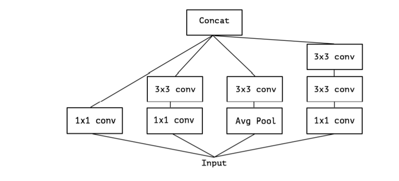
Inception 스타일 모델의 기본적인 building block은, 여러 버전이 존재하는 Inception module이다.Fig.1에서는 canonical Inception module Inception-v3에서 볼 수 있는 표준 형태의 Inception module을 보여준다.Inception 모델은 이러한 모듈들의 stack으로 이해할 수 있다. 이것은 simple convolution layers의 스택이었던 이전 VGG-style networks에서 출발 한 것이다.

 

Inception module은 개념적으로 convolutions (they are convolutional feature extractors)과 유사하지만, 실험에서는 적은 parameter로도 풍부한 표현을 학습할 수 있는 것으로 나타났다. 이들은 어떻게 작동하며, 일반적인 convolution과 어떻게 다른 것일까? Inception 이후에는 어떤 디자인 전략이 나올까?

 

1.1. The Inception hypothesis

Convolution layer는 2개의 spatial dimension(width and height)과 channel dimension로 이루어진 3D 공간에 대한 filter를 학습하려고 시도한다. 따라서 single convolution kernel은 cross-channel correlation과 spatial correlation을 동시에 mapping하는 작업을 수행한다.

 

Inception module의 기본 아이디어는 cross-channel correlation과 spatial correlation을 독립적으로 볼 수 있도록 일련의 작업을 명시적으로 분리함으로써, 이 프로세스를보다 쉽고 효율적으로 만드는 것이다. 더 정확하게 , 일반적인 Inception module의 경우, 우선 1x1 convolution으로 cross-correlation을 보고, input보다 작은 3~4개의 분리 된 공간에 mapping한다. 그 다음 보다 작아진 3D 공간에 3x3 혹은 5x5 convolution을 수행하여 spatial correlation을 mapping한다. Fig 1 참조 . 실제로 Inception의 기본 가설은 cross-channel correlations 과 spatial correlations는 충분히 분리되어 공동으로 매핑하지 않는 것이 좋다. 

 

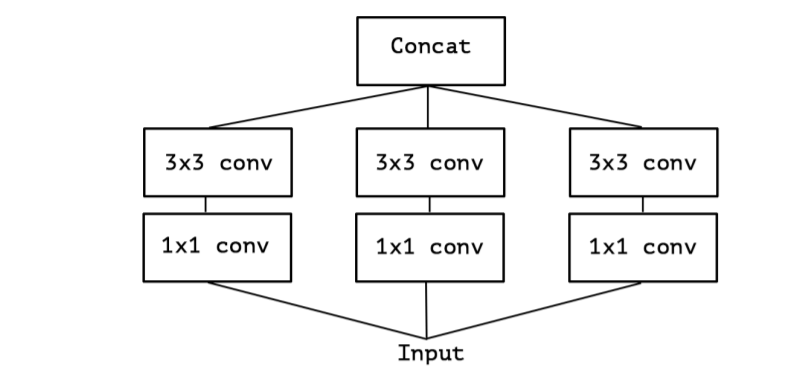
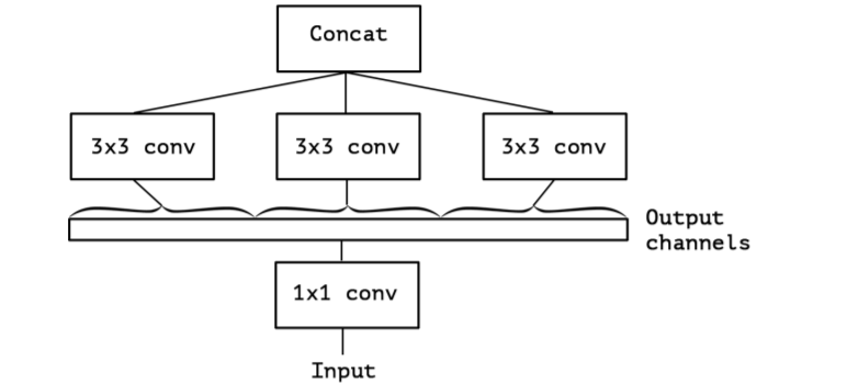
convolution (e.g. 3x3)를 하나만 사용하고 average pooling tower (figure 2)을 포함하지 않는 simplified 버전의  an Inception module를 고려한다. 이 Inception module은 a large 1x1 convolution을 수행하고 , output channels (figure 3)

들의 겹치지 않는 segment에 대한 spatial convolutions이 오는 형태로 재구성한다. 이 관찰은 자연스럽게 다음의 문제를 제기한다 :  Partition 내의 segment 개수나 크기가 어떤 영향을 갖는가? nception의 가설보다 훨씬 강력한 가설을 세우고, cross-channel correlation과 spatial correlation을 완전히 분리시켜 mapping 할 수 있다고 가정하는 것이 합리적인가?

Figure 1. A canonical Inception module (Inception V3).

Figure 2. A simplified Inception module.

Figure 3. A strictly equivalent reformulation of the simplified Inception module.

Figure 4. An “extreme” version of our Inception module, with one spatial convolution per output channel of the 1x1 convolution.

1.2. The continuum between convolutions and separable convolutions

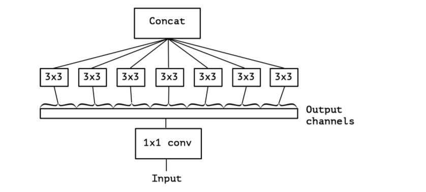
“extreme” version of an Inception module 강렬한 가설의 기반으로 , 우선 우리는 1x1 convolution으로 cross-channel correlations 매핑하고 , 각각의 output channel 들의 spatial correlations을 따라 매핑한다. figure 4에서 볼 수 있다. We remark that this extreme form 의 an Inception module 이 depthwise separable convolution 거의 almost identical 하며 , an operation that has been used in neural network design as early as 2014 [15] and has become more popular since its inclusion in the TensorFlow framework [1] in 2016. 

 

depthwise separable convolution는  deep learning frameworks such as TensorFlow and Keras에서  일반적으로 “separable convolution”부르며 , depthwise convolution으로 구성된다. 즉 input의 각 channel에 대해 , 독립적으로 , a spatial convolution이 수행되고 , 그 뒤로는 pointwise convolution 따라오는 형태이다. 1x1 convolution은 depthwise convolution 의 output을 새로운 channel space 에 projecting한다. spatially separable convolution과 혼동되서는 안되며 image processing community에서는 일반적으로 “separable convolution”라고 한다.

 

“extreme” version의 Inception module과 depthwise separable convolution 간의 두가지 차이점은 아래와 같다.

operations의 순서 : Inception에서는 1x1 convolution을 먼저 수행하는 반면, 예를 들면 TensorFlow에서와 같이 일반적으로 구현된 depthwise separable convolution은 channel-wise spatial convolution을 먼저 수행한 뒤에 1x1 convolution을 수행한다.

첫 번째 operation 뒤의 non-linearity presence or absence . Inception에서는 두 operation 모두 non-linearity로 ReLU가 뒤따르는 반면, separable convolution은 일반적으로 non-linearity 없이 구현된다.

우리는 operation들이 stacked setting에서 사용되기 때문에, 첫 번째 차이점은 중요하지 않다고 주장한다. 두 번째 차이점은 중요할 수 있으므로 실험 파트에서 조사한다.(in particular see figure 10)

 

또한 , 일반  Inception module 과 depthwise separable convolutions 사이의 intermediate formulations도 가능함에 주목한다. 사실은, there is a discrete spectrum between regular convolutions and depthwise separable convolutions, parametrized by the number of independent channel-space segments used for performing spatial convolutions.

일반적인 convolution , (preceded by a 1x1 convolution) , at one extreme of this spectrum,  single-segment case에 해당한다;  a depthwise separable convolution channel당 하나 해당한다; Inception modules은 수백개의 channel을 3 or 4 segments 다루기 때문에 이 둘 사이에 있다. 

 

이러한 관측으로 부터 우리는 Inception modules을 depthwise separable convolutions으로 대체함으로써 Inception family 의 구조를 개선하는 것이 가능할 것이라 제안한다. i.e. depthwise separable convolution을 stacking한 모델을 building 한다. 이는 Tensorflow에서 사용할 수 있는 효율적인 depthwise separable convolution으로 실현된다. 다음에서 우리는 이 아이디어를 기반으로  Inception V3와 유사한 수의 매개 변수 를 사용하는 convolutional neural network architecture를 제시하고  ,  two large-scale image classification task Inception V3에 대한 성능을 평가한다.

 

2. Prior work

이 연구는 다음 분야의 이전 연구들에 크게 의존한다.

• Convolutional neural networks [10, 9, 25], 특히  VGG-16 architecture [18] 는 몇 가지 측면에서 우리가 제안한 아키텍처와 개략적으로 유사하다.

• The Inception architecture family of convolutional neural networks [20, 7, 21, 19], 여러개의  branches 로 factoring하여 ,channel들과 이 공간에서 연속적으로 등장하는 것에 대한  중점을 두었다.

 

• Depthwise separable convolutions는 아키텍처가 전적으로 기반으로 제안되였다. 네트워크에서 spatially separable convolution이 사용됐던건 2012[12] (but likely even earlier) 년 이전이지만, depthwise version은 더 최근에 사용됐다. Laurent Sifre는 2013년에 Google Brain internship 과정에서 depthwise separable convolution을 개발했으며, 이를 AlexNet에 적용하여 큰 수렴 속도 향상과 약간의 성능 향상, 모델 크기의 감소 등의 성과를 얻었다. 그의 작업에 대한 개요는 ICLR 2014[23]에서 처음 공개되었다. 자세한 실험결과는 Sifre’s thesis, section 6.2 [15]에서 보고됐다.Depthwise separable convolution에 대한 초기 연구는, Sifre and Mallat on transformation-invariant scattering [16, 15]에서 영감을 받았으며, 이후에는 depthwise separable convolution이 Inception V1와 Inception V2 [20, 7]의 첫번째 레이어에 사용되였다. Google의 Andrew Howard [6] 는 depthwise separable convolution을 사용하여 MobileNets이라는 효율적인 모바일 모델을 도입했다. Jin et al. in 2014 [8] and Wang et al. in 2016 [24] 연구에서도 separable convolution을 사용하여 CNN의 크기 및 계산 비용을 줄이는 연구를 수행했다. 또한 우리의 작업은 TensorFlow 프레임 워크에 깊이 별 분리 가능한 컨볼 루션을 효율적으로 구현 한 경우에만 가능하다 [1].

 

• Residual connections, introduced by He et al. in [4], which our proposed architecture uses extensively.

 

3. The Xception architecture

우리는 전적으로 depthwise separable convolution layers에 기반한 convolutional neural network구조를 기반으로 제안한다. 사실은 다음과 같은 가설을 세운다. convolutional neural networks의 feature maps에서 cross-channels correlations and spatial correlations의 mapping 은 완전히 분리될수 있다. 이는 Inception 구조에 기반한 강력한 버전의 가설이므로, 제안하는 구조를 “Extreme Inception“을 나타내는 이름인 Xception으로 명명한다.

 

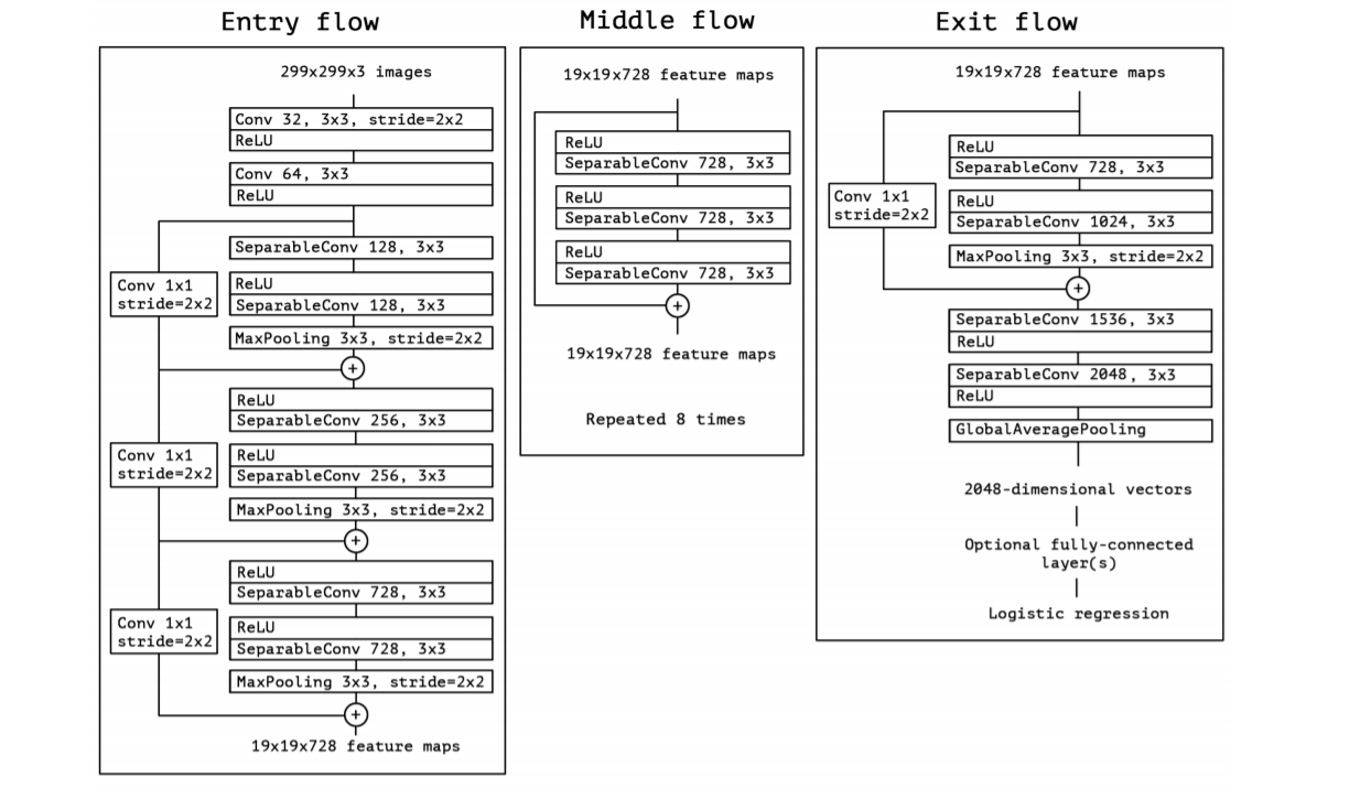
network에 대한 자센한 정보는 figure 5를 참조한다. Xception 구조는 36개의 conv layer로 feature extraction을 수행한다. 실험 평가에서는 image classification에 대해서만 조사하므로, 제안하는 CNN에는 logistic regression layer가 뒤따른다.선택적으로 logistic regression layer 앞에 완전히 연결된 계층을 삽입 할 수 있다.이것은 experimental evaluation section (in particular, see figures 7 and 8)에 나와있다. 36개의 conv layer는 14개의 모듈로 구성되며, 첫 번째와 마지막 모듈을 제외한 나머지의 주위에는 linear residual connection이 있다.

 

간단하게 말하자면 ,  Xception 구조는 residual connection이 있는 depthwise separable convolution의 linear stack으로 볼 수 있다. 따라서 Xception 구조는 정의와 수정이 매우 쉽게 이루어질 수 있다. Keras [2] 나 TensorFlow-Slim[17] 과 같은 high-level library를 사용하면 30~40줄의 코드로 구현이 가능하다. VGG-16[18]이나 훨씬 복잡한  Inception-v2혹은 Inception-v3과는 차이가 있다. 오픈 소스 구현은 Keras 애플리케이션 모듈 , MIT 라이센스에 따라 Keras 및 TensorFlow를 사용하는 Xception은 다음의 일부로 제공된다. 

 

4. Experimental evaluation

우리는 규모의 유사성을 고려해 , Xception to the Inception V3 architecture 비교한다. Xception과 Inception-v3의 parameter 수는 거의 동일하므로, 성능 차이는 네트워크 capacity의 차이에서 비롯된 것이 아니다. (Table.3 참조) 우리는 성능은 두 개의 image classification task에 대해 비교한다. 하나는 우리가 알고있는 1000-class single-label classification task on the ImageNet dataset [14], 또 다른 하나는 17,000-class multi-label classification task on the large-scale JFT dataset.

 

4.1. The JFT dataset

JFT는 large-scale image classification dataset을 위한  internal Google dataset  으로, Hinton et al. in [5] 처음으로 도입했다. 데이터는 17000-class label로 분류 된 350 million 의 고해상도 이미지로 구성된다.  JFT에 대해 학습 된 모델의 성능 평가를 위해, 보조 dataset인 FastEval14k를 사용한다.

 

FastEval14k is a dataset of 14,000 images with dense annotations from about 6,000 classes (36.5 labels per image on average).  이 dataset에서는 top-100 prediction에 대한 Mean Average Precision(이하 MAP@100)으로 성능을 평가하고, MAP@100의 각 class에 기여도를 가중치로 부여하여, 소셜 미디어 이미지에서 해당 class가 얼마나 흔하게 사용되는지 추정한다.이 평가 절차는 소셜 미디어 이미지에서 자주 발생하는 label의 성능을 측정하기 위한 것으로, Google의 production models에 중요하다고 한다.

 

4.2. Optimization configuration

ImageNet과 JFT에서는 서로 다른 optimization configuration을 사용했다.

• On ImageNet:

– Optimizer: SGD

– Momentum: 0.9

– Initial learning rate: 0.045

– Learning rate decay: decay of rate 0.94 every 2 epochs

• On JFT:

– Optimizer: RMSprop [22]

– Momentum: 0.9

– Initial learning rate: 0.001

– Learning rate decay: decay of rate 0.9 every 3,000,000 samples

 

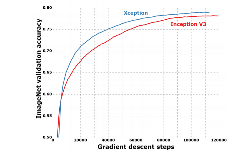
두 dataset 모두, Xception과 Inception-v3에 동일한 optimization configuration이 사용됐다.이 configuration은 Inception-v3의 최고 성능에 맞춘 것이며, Xception에 최적화 된 hyperparameter로 조정하려는 시도를 하지 않았다. 두 네트워크의 학습 결과가 다르기 때문에, 특히 ImageNet dataset에서는 Inception-v3에 맞춰진 configuration이 최적값이 아닐 수 있다. (Fig.6 참조) 

 

모든 모델은 inference time에 Polyak averaging [13] 을 사용하여 평가된다.

 

4.3. Regularization configuration

 

• Weight decay:

Inception-v3은 rate가 4e-5인 weight decay(L2 regularization)를 사용하여, ImageNet의 성능에 맞게 신중하게 조정됐다. Xception에서는 이 rate가 매우 부적합하기 때문에, 1e-5를 사용한다.우리는 Optimal weight decay rate에 대한 광범위한 탐색은 하지 않았으며, ImageNet과 JFT에 대한 실험 모두에서 동일한 weight decay rate가 사용됐다.

 

• Dropout:

ImageNET 실험의 경우  , 두가지 모델의 dropout layer of rate 0.5 before the logistic regression layer포함한다 . JFT 실험의 경우, dataset의 크기를 고려하면 적절한 시간 내에 overfitting 될 수가 없으므로 dropout이 포함되지 않는다.

 

• Auxiliary loss tower:

Inception-v3 아키텍처에서는 네트워크의 초반부에 classification loss를 역전파하여, 추가적인 regularization 메커니즘으로 사용하기 위한 auxiliary loss tower를 선택적으로 포함할 수 있다. 단순화를 위해, auxiliary tower를 모델에 포함하지 않기로 했다.

 

4.4. Training infrastructure

모든 networks 의 TensorFlow framework [1] 구성했으며  NVIDIA K80 GPUs 에서 60가지를 학습하였다. ImageNet 실험의 경우, 최상의 classification 성능을 달성하기 위해 synchronous gradient descent과 data parallelism을 이용했으며, JFT의 경우에는 학습 속도를 높이기 위해 asynchronous gradient descent를 사용했다. ImageNet에 대한 실험은 각각 약 3일이 걸렸고, JFT에 대한 실험은 1개월이 넘게 걸렸다. JFT 모델 에 대해 full convergence로 학습하려면 3개월씩 걸리기 때문에, 이렇게까지 학습하진 않았다고 한다.

Figure 5. The Xception architecture: the data first goes through the entry flow, then through the middle flow which is repeated eight times, and finally through the exit flow. Note that all Convolution and SeparableConvolution layers are followed by batch normalization [7] (not included in the diagram). All SeparableConvolution layers use a depth multiplier of 1 (no depth expansion).

4.5. Comparison with Inception V3

4.5.1 Classification performance

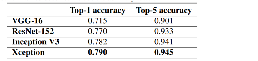
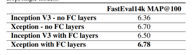
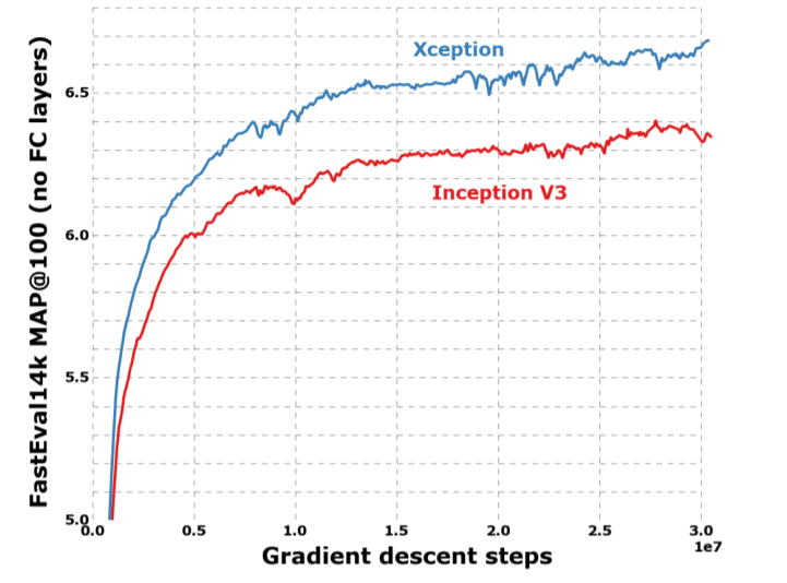
모든 평가는 single crop과 single model에 대해 수행됐다.ImageNet에 대한 결과는 test set이 아닌 validation set에 대해 측정됐다. (Table.1, Fig.6 참조) JFT에 대한 결과는 full convergence 후가 아닌  30 million회의 iteration (one month of training)후에 측정됐다.  결과는 in table 1 and table 2, as well as figure 6, figure 7, figure 8 에 있다. 우리는  JFT에서는 fully-connected layer가  포함되지 않은 버전과, logistic regression layer 이전에 4096개의 노드로 이루어진 fully-connected layer가 2개 포함 된 버전을 테스트했다.

 

ImageNet에서 Inception V3은 Xception보다  약간 더 나은 결과를 보여준다. JFT에서의 Xception은 FastEval14k에 대한 MAP@100에서 4.3%의 상대적 개선을 보여줬다. 또한 Xception은, ResNet에서 보고 된 ResNet-50, ResNet-101, ResNet-152의 ImageNet classification 성능보다 우수하다.

Table 1. Classification performance comparison on ImageNet (single crop, single model). VGG-16 and ResNet-152 numbers are only included as a reminder. The version of Inception V3 being benchmarked does not include the auxiliary tower

Xception 아키텍처는 ImageNet dataset보다 JFT dataset에 대해 더 큰 성능 향상을 보여줬다. 이는 Inception-v3가 ImageNet dataset에 중점을 두고 개발됐기 때문에, 디자인이 특정 작업에 과적합 된 것으로 볼 수 있다. 즉, ImageNet dataset(부분적인 optimization parameters 와 regularization 파라미터들 )에 더 적합한 hyperparameter를 찾는다면 상당한 추가적 성능 향상을 얻을 수 있을거라 볼 수 있다.

 

Table 2. Classification performance comparison on JFT (single crop, single model).

Figure 6. Training profile on ImageNet

Figure 7. Training profile on JFT, without fully-connected layers

4.5.2 Size and speed

Table 3. Size and training speed comparison.

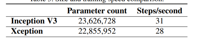
table 3에서 우리는 Inception V3 와  Xception 사이즈 및 속도에 대해 비교한다. Parameter의 개수는 ImageNet(1000 가지 종류, fully-connected layers가 없다. )에 대한 학습 모델에서 측정됐으며, 초당 training step(gradient update)은 ImageNet dataset에 대한 synchronous gradient descent 횟수를 측정했다. 두 모델의 크기 차이는 거의 같으며(약 3.5% 이내로), 학습 속도는 Xception이 약간 느린 것으로 나타났다. 두 모델이 거의 동일한 수의 parameter를 가지고 있다는 사실은, ImageNet과 JFT에 대한 성능 향상이 capacity의 증가가 아니라, 모델의 parameter를 보다 효율적으로 사용함으로써 이뤄졌다는 것을 나타낸다.

 

4.6. Effect of the residual connections

Figure 9. Training profile with and without residual connections.

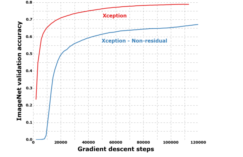
Xception 구조에서의 residual connection 효과를 정량화하기 위해, residual connection을 포함하지 않는 버전의 Xception을 ImageNet에 대해 벤치마크했다. 결과는 figure 9에서 참조한다. 수렴 속도나 최종 classification 성능 측면에 있어, residual connection은 반드시 필요한 것으로 보여진다. 물론, residual 버전과 동일한 optimization configuration으로 non-residual 버전을 벤치마킹했기 때문에 차이가 더 크게 나온 것일 수도 있다.

 

추가적으로 , 이 결과는 Xception에서 residual connection의 중요성을 보여준 것일 뿐이지, depthwise separable convolution의 stack인 이 모델의 구축에 필수 조건은 아니다. 또한, non-residual VGG-style 모델의 모든 conv layer를 depthwise separable convolution(with a depth multiplier of 1)으로 교체했을 때, 동일한 parameter 수를 가지고도 JFT dataset에서 Inception-v3보다 뛰어난 결과를 얻었다.

 

4.7. Effect of an intermediate activation after pointwise convolutions

Figure 10. Training profile with different activations between the depthwise and pointwise operations of the separable convolution layers.

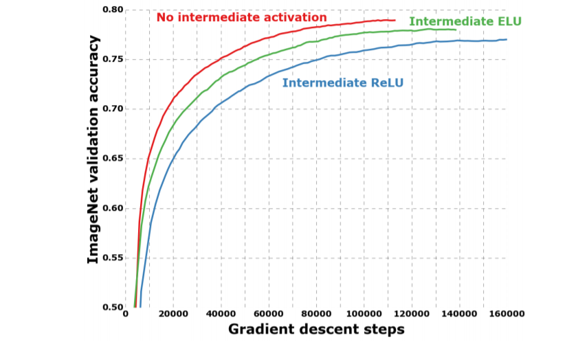
우리는 전에서 depthwise separable convolution과 Inception module의 다른 점이, depthwise separable convolution의 depthwise operation과 pointwise operation 사이에 non-linearity를 포함해야할 수도 있음을 시사한다고 언급했었다. 지금까지의 실험 파트에서는 non-linearity가 포함되지 않았다. 이 절에서는 intermediate non-linearity로 ReLU 또는 ELU [3]의 포함 여부에 따른 효과를 실험적으로 테스트한 결과를 보인다. ImageNet에 대한 실험 결과는 Fig.10에 보이듯, non-linearity가 없으면 수렴이 빨라지고 최종 성능도 향상됐다.

 

이는 Inception module에 대한 Szegedy et al.와 반대되는 놀라운 관찰이다. 이는 spatial convolution이 적용되는 intermediate feature space의 depth가 non-linearity의 실용성에 매우 중요하게 작용되는 것으로 볼 수 있다: 즉, Inception module에 있는 deep feature space(e.g. those found in Inception modules)의 경우에는 non-linearity가 도움이 되지만, shallow feature space (e.g. the 1-channel deep feature spaces of depthwise separable convolutions)의 경우에는 오히려 정보 손실로 인해 해로울 수가 있다.

 

5. Future directions

우리는 전에서 일반적인 convolution과 depthwise separable convolution 간에는 별개의 스펙트럼이 존재한다고 언급했었다. Inception module은 이 스펙트럼의 한 지점에 해당한다. 우리는 실험적인 평가에서 Inception module의 extreme formulation 인 depthwise separable convolution이 일반적인 Inception module보다 이점을 가질 수 있음을 보여줬지만, depthwise separable convolution이 optimal이라고 믿을 이유는 없다.일반적인 Inception module과 depthwise separable convolution의 스펙트럼 사이에 위치한 아키텍처가 추가적인 이점을 가질 수도 있다. 이는 향후 연구를 위해 남겨졌다.

 

6. Conclusions

Convolution과 depthwise separable convolution이 어떻게 양 극단의 스펙트럼에 놓여 있는지를 보여줬다. Inception module은 둘의 중간 지점에 위치한다. 이러한 관찰에 따라, 컴퓨터 비전 아키텍처에서 Inception module을 depthwise separable convolution으로 대체 할 것을 제안했다.이 아이디어를 기반으로 Xception이라는 새로운 아키텍처를 제시했으며, 이는 Inception-v3과 유사한 수의 parameter를 갖는다. Xception을 Inception-v3과 성능을 비교했을 때, ImageNet dataset에 대해서는 성능이 조금 향상됐으며, JFT dataset에 대해서는 성능이 크게 향상됐다. 우리는 Depthwise separable convolution은 Inception module과 유사한 속성을 지녔음에도 일반 conv layer만큼 사용하기가 쉽기 때문에, 향후 CNN 아키텍처 설계의 초석이 될 것으로 기대된다.

 

 

 

Depth-wise-separable convolution

depth-wise separable convolution 연산은 각 채널 별로 convolution 연산을 시행하고 그 결과에 1x1 convolution 연산을 취하는 것이다. 기존의 convolution이 모든 채널과 지역 정보를 고려해서 하나의 feature map을 만들었다면, depthwise convolution은 각 채널 별로 feature map을 하나씩 만들고, 그 다음 1x1 convolution 연산을 수행하여 출력되는 피쳐맵 수를 조정한다. 이 때의 1x1 convolution 연산을 point-wise convolution이라 한다.

 

https://www.youtube.com/watch?v=T7o3xvJLuHk

 

 

 

 

[논문] : Xception Deep Learning with Depthwise Separable Convolutions

[참고]

https://sike6054.github.io/blog/paper/fifth-post/

(Xception) Xception: Deep Learning with Depthwise Separable Convolutions 번역 및 추가 설명과 Keras 구현

https://wingnim.tistory.com/104

Depthwise Separable Convolution 설명 및 pytorch 구현

https://datascienceschool.net/view-notebook/0faaf59e0fcd455f92c1b9a1107958c4/

Data Science School