[Image Classification] LeNet5 : Gradient-Based Learning Applied to Document Recognition

[논문]:Gradient-Based Learning Applied to Document Recognition

LeNet5 

 

LeNet5  간단하게 요약  :

모델 구조 

Convolutional Neural Network 

subsmapling 

우편번호와 필기체 인식하기 위한

 

XI. Conclusions

학습

CNN을 통해 직접 특징 추출하는 것을 할 필요 없게 되었음.

GTN을 통해 파라메터 튜닝, 레이블링, 경험에 의존한 방법들의 사용을 줄일 수 있었음.

학습할 데이터가 많아지고 , 컴퓨터도 빨라졌다.

그래서 학습이 중요하다. 

 

bACK-propagation algorithm

multi-ayer neural networks

gradient-based learning  for Graph transformer Netorks

 

Maximum Likelihood Principle

 

해당 GTN은 전체적인 성능 향상을 위해 여러 모듈들에 대해 Gradient 기반 학습을 하도록 합니다.
GTN에 대해 대략적으로 읽어본 결과, 수표 인식을 위해 캐릭터 하나 하나를 분할하기 위한 방법에 대해 설명하는 내용이었습니다

1. Feature extration 전통저긍로 fixed transform

2. segmentation and recognition of objects in image cannot be compeletely decoupled.

3. Hand truthing images to obtain segmented characters for training a character recognizer  is expensive and does not take into account the way in which a whole document or sequence of characters will be recognized.

4. Ambiguities inherent in the segmentation, character recognition, and linguistic model should be integrated optimally.

5. traditional recognition systems rely on many hand-crafted heuristics to isolate  individually recognizable objects.

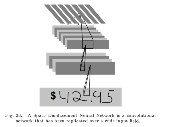
Space Displacement Neural Network

 

Abstract--

Gradient-Based Learning Technique  

back-propagation algorithm  -> gradient-based learning technique  ->high-dimensional patterns

이 논문은 다양한 방법으로 handwriten character recognition 를 지원하고 표준화 손글때 digit recognition 을 비교하는 작업이다.

Graph Transformer Networks:

주요한 역할은 original image에서 아직 연결되지 않는 노드들의 유용한 연결을 식별한다.

Two systems for on-line handwriting recognition

experiments demonstrate global training

GTN: flexibility  bankcheck 

 

1. Introduction 

pattern recognition systems

이 논문에서의 주오한 메시지는 

better pattern recognition systems can be built by relying more on automatic learning, and less on hand-designed heuristics.

 

End-to-end & Hand-crafted

End-to-end : input original data , output result

Hand-crafted: End-to-end와 대비된다. 사람이 수동으로 설계하여 한 step 마다 step마다 설명이 가능한 것이다.

 

character recoginition as a case study -> hand-crafted feature extraction

document understanding as a case stuty-> GTN

GTN : that allow training all the modules to optimize a global performance criterion

 

most pattern recognition systems are built using a combination of automatic learning techniqes and hand-crafted algorithms.

recognizing individual patterns consists in dividing the system into two main moduls

first module, feature extractor, transforms the input patterns so that they can be represented by low-dimensional vectors or short strings of sysmbols 

(a) can be easily matched or compared

(b) relatively invariant with respect to transformations and distortions of the input patterns that do not change their nature.

feature extractor : contains most of the prior knowledge and is rather specific to the task. It is also the focus of most of the design effort, because it is often entirely hand-crafted.

classifier , general-purpose and trainable.

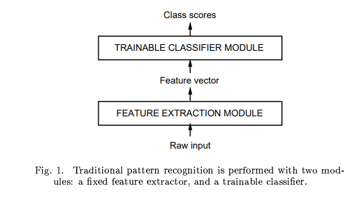
1. 특징 추출

Raw input-> Feature vector(특징을 추출한다.)->class scores(거의 변하지 않는다.)

특징 추출이 어렵다.

feature extractors

a combination of three factors have changed this visin over the last decade

1. the availability of low-cost machines with fast arithmetic units allows to rely more on brute-force "numerical" methods than on algorithmic refinements =>계산

2. the availability of large databases for problems with a large market and wide interest, such as handwriting recognition, has enabled designers to rely more on real data and less on hand-crafted feature extraction to build recognition systems => databases

3. 매우 중요한 요인 is the avilability of powerful machine learning techniques that can haldle high-dimensinal inputs and can generate intricate decision functions when fed with these large data sets. => high-dimensional

 

OCR systems use some form of multi-layer Neural Network trained with back-propagation.

 

multi-layer neural network

Convolutional Neural  Network

LeNet-5 -> this system is in commercial use in the NCR Corporation line of check recognition systems for the baking industry.

 

Section 소계 :

 

A. Learning froam Data'

이미지는 크다. pixel로 구성되였다. 수천 만 개 의 weight가 있다. 

"numerical" or gradient-based learning

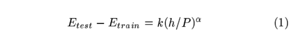
P is the number of training samples, 

h is a measure of "effective capacity" or complexity of the machine Statistical Learning

알파 is a number between 0.5 and 1.0 and k is a constant.

h increace Etrain decreases  

Etrain줄이는 목적으로 한다.

 

In practical terms, Structural Risk Minimization is implemented by minimizing

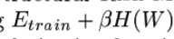
H(W) IS called a regularization fuction 

베타 is constant

H(W) is chosen such that it takes large values on parameters W that belong to high-capacity subsets of the parameter space.

minimizing H(W) in effect limits the capacity of the accessible subset of the parameter space, 

ghereby controlling the tradeoff between minimizing the training error and minimizing the 

expected gap between the training error and test error.

에러를 줄여야 한다. 

 

B. Gradient-Based Learning => loss fuction

Efficient learning algorighms can be devised when the gradient vector can be computed analytically

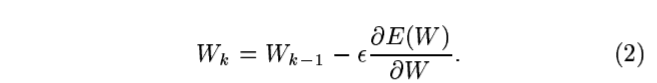
W is a real-valued vector, with respect to which E(W) is continuous, as well as differentiable almost ererywhere

 a popular minimization procedure is the stochastic gradient algorithm -> online updatae

C. Gradient Back-Propagation

the suprising usefulness of such simple gradient descent techniques for complex machine learning tasks was not widely realized unitil the following three events occurred.

1. realization ,  loss function 은 학습할떄 중요한 원인이 아니다.

2. back-propagation algorighm, to compute the gradient in a non-linear systen compused of several layers of processing. 

3. back-propagation procedure applied to multi-layer neural networks with sigmoidal units can solve complicated learning tasks.

기울기 줄이는 것 

 

back-propagation

 

D. Learning in Real Handuriting Recoginition Systems

Gradient-Based Learning 

Convolutional Netwoks

The best neural networks , called Convolutional Networks , are designed to learn to extract relevant features directly from pixel images

Heuristic over-segmentation:

은닉 마르코프 모형(영어: hidden Markov model, HMM)은 통계적 마르코프 모형의 하나로, 시스템이 은닉된 상태와 관찰가능한 결과의 두 가지 요소로 이루어졌다고 보는 모델이다. 

마르코프 모형 - 위키백과, 우리 모두의 백과사전

label 등 

 

training the system at the level of whole strings of characters, rather than at the chracter level

eliminate segmentation altogether

 

 

E. Globally Trainable Systems

multiple modules.

 

Convolutianal Neural Networks for isolated character recognition

a trainable classifier then categorizes the resulting feature vectors into classes.

in this scheme, standard, fully-connected multi-layer networks can be used as classifiers.

 

1. typical images are large, often with several hundred variables(pixels).

100개 의 hidden units in the first layer,  수많은 weights가 있다.

capacity -> memory 

2. a deficiency of fully-connected architectures is that the topology of the input is entirely ignored.

convolutional networks force the extraction of local features by restricting the receptive fields of hidden units to be local

 

A. Couvolutional Networks

Convolutioanl Networks combine three architectural ideas to ensure some degree of shift, scale, and distortion invariance: 3가지 구조 

local receptive fields,

shared weights(or weight replication)

spatial or temporal sub-sampling.

 

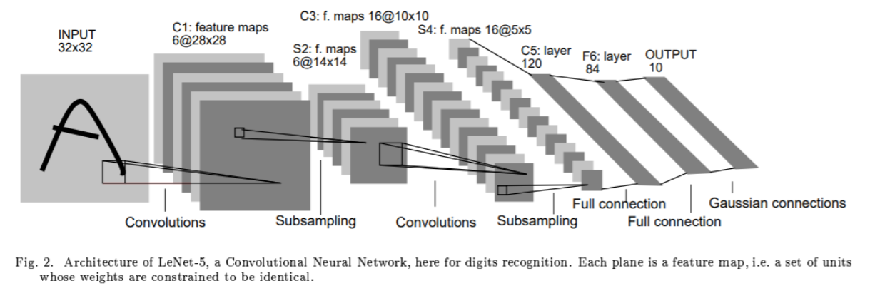
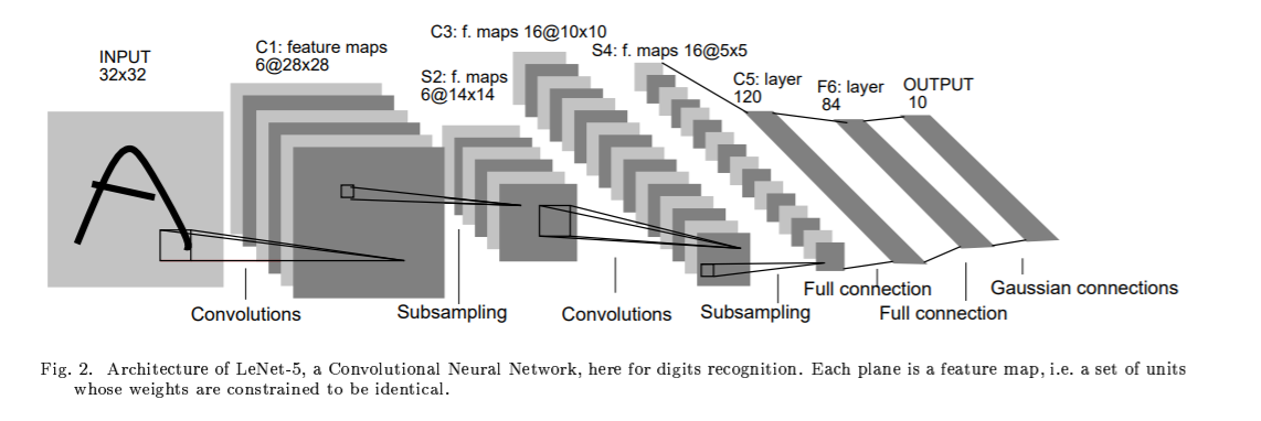
LeNet-5 구조

the input plane receives images of characters that are appoximately size-normalized and centered.

each unit in a layer receives inputs from a set of units located in a small neighborhood in the previous layer.

 

subsampling:  출력의 일부분만 취하는 것이다.

6 planes

gas 25 uboyts cibbected ti a 5x5

 

feature map

 

 

B. LeNet-5 구조 

7 layers (not couting the input)

input 32x32 pixel image

hight-level feature detectors.

 

Cx: convolutional layers

Sx: subsampling layers 

Fx: fully-connected layers

x : layer index.

 

layer C1 : covolutional layer with 6 feature maps.

Each unit in each feature map is connected to a 5x5 neightborhood in input

The size of the feature map is 28x28 which prevents connection from the input from falling off the boundary

파라미터 156 , 그리고 122,304 개 연결되여있다.

 

layer S2 sub-sampling layer with 6 feature maps of size 14x14 .

Each unit in each feature map is connected to a 2x2 neighborhood in the corresping feature map in C1.

2x2 receptive fields are non-overlapping

 

layer C3 : covolutional layer with 16 feature maps.

ach unit in each feature map is connected to a 5x5 neightborhoodS at identiacal locations in a subset of S2's feature maps.

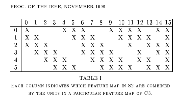
Table1 . shows the set of S2 feature maps conbined by each C3 feature map.

 

Why not connect every S2 feature map to every C3 feature map?

the reason is twofold.

a non-compelete connection scheme keeps the number of connections within reasonable bounds. 더 중요한것은 이미지의 대칭을 깬다. different feature maps are foreced to extract different(hopefully complementary) features because they get differnt sets of inputs. 

the 처음의 6개 feature maps take inputs from every contiguous subsets of three feature maps in S2.

다음의 6개는 take input from every contiguous subset of four

finally the last one takes input from all S2 feature maps.

1,516 trainable parameters and 151,600 connections

 

layer S4 subsampling layer with 16 feature maps of size 5x5 

32 trainable parameters and 2,000 connections

 

Layer C5 is a convolutional layer with 120 feature maps.

feature map is 1x1

C5 is labeled as a convoluional layer, instead of a fully-connected layer, because if LeNet-5 input were made bigger with everything else kept constant, the feature map dimension would be larger than 1x1.

48,120 trainable connections

 

Layer F6, contains 84 units. 10,164 trainable parameters.

classical neural networks , units in up to F6 compute a dot product between their input vector and their weight vector, to which a bias is added.

 

RBF: Radial Basis Function units

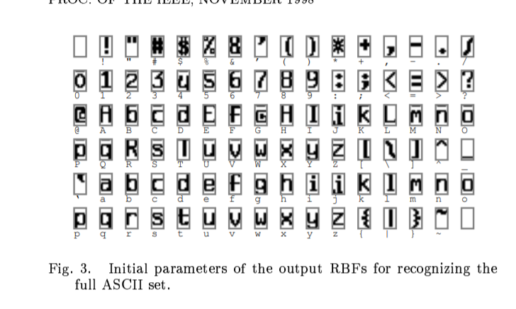
그림 초기화 파라미터 -> output RBFs 

layer output layer: 10 classes, 0-9 , softmax

 

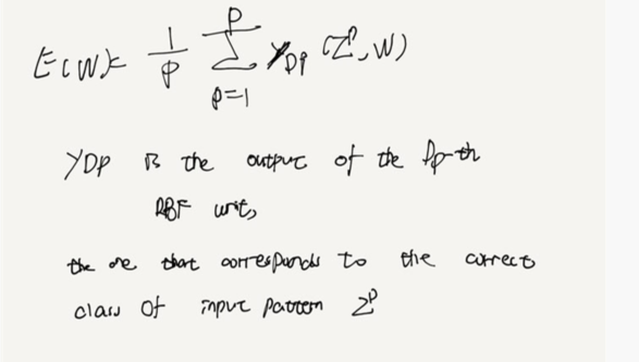
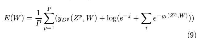
C.Loss function

Maximum Likelihood Estimation criterion 

Minimum Mean Squared Error(MSE)

 

Results and Comparison with other methods 결과에 대한 비교

A. database: the modified NIST set -> MNIST

B. Results

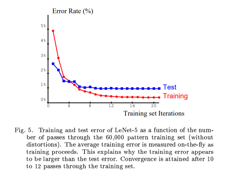
학습 에러가 테스트 에러 보다 크다. 

transformations: horizontal and vertical translations, scaling, squeezing(simultaneous horizontal compression and vertical elonggation, or the reverse) and horizontal shearing.

 

비뚤어진 패턴으로 학습을 하였다. 정확도가 떨어진다. 0.95% -> 0.8%

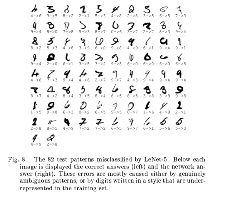
misclassified test examples

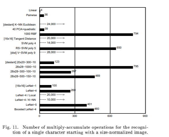
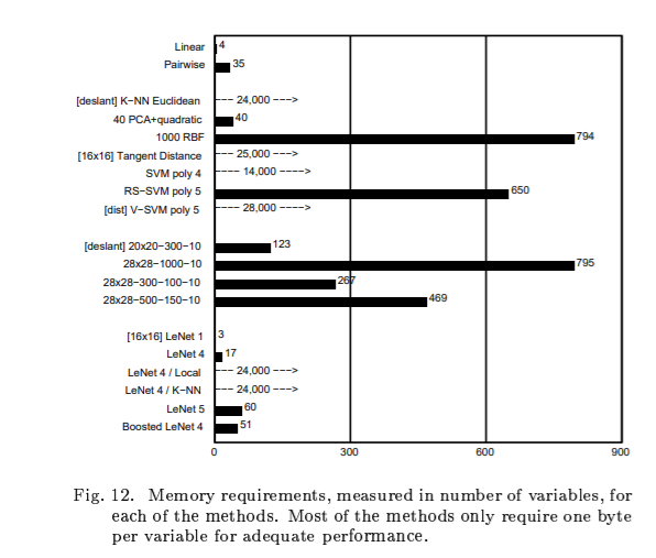
C. Comparison with Other Classifiers

C.1 Linear Classifier, and Pairwise Linear Classifier

Linear Classifier 선형 분류 : Each input pixel value contributes to a weighted sum for each output unit.

The output unit with the hightest sum(including the contribution of a bias constant) 

error rate is 12% 8.4% 7.6%

 

C.2 Baseline Nearest Neighbor Classifier

K-nearest neighbor classifier 

메모리가 많이 필요하다.

Euclidean distance

 

C.3 Pricinpal Component Analysis(PCA) and Polynomial Classifier

C.4 Radial Basis Function Network

C.5 One-Hidden Layer Fully Connected Multilayer Neural Network

C.6 Two-Hidden Layer Fully Connected Multilayer Neural Network

C.7 A Small Convolutional Network: LeNet-1

The images down-sampled to 16x16 pixels and centered in the 28x28 input layer

C.8 LeNet-4

C.9 Boosted LeNet-4

C.10 Tangent Distance Classifier(TDC)

nearest-neighbor mehod where the distance function is made in-sensitive to small distortions and translations of the input image

C.11 Support Vector Machine(SVM)

D. discussion

E. Invariance and Noise Resistance

 

 

Multi-Module Systems and graph Transformer networks

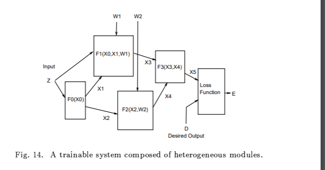
A. An Object-Oriented Approach

"backward propagation"

"forward propagation

 

B. Special Modules

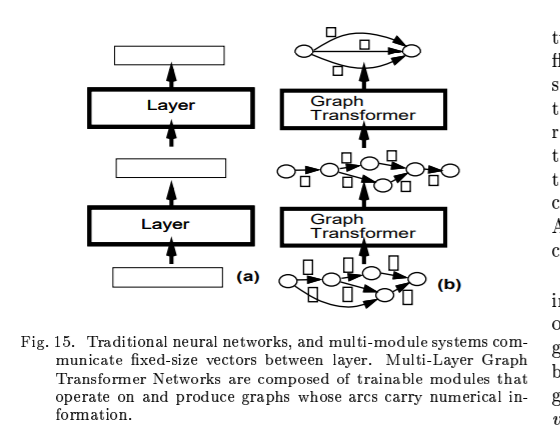
C. Graph Transformer Networks

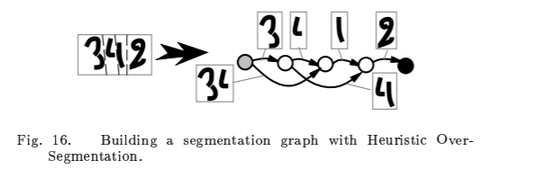
Multiple Ojbect Recogniton: Heuristic Over-Segmentation

 

A. segmentation Graph

B. Recognition Transformer and Viterbi Transformer

Global Training for graph transformer networks

 

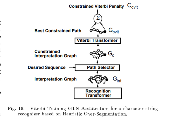
A. Viterbi Training

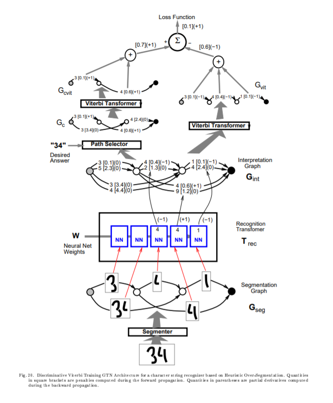
B. Discriminative Viterbi Training

C. Forward Scoring, and Forward Training

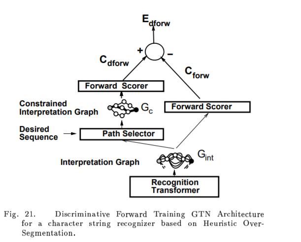
D. Discriminative Forward Training

E. Remaks Discriminative Training

 

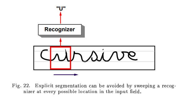
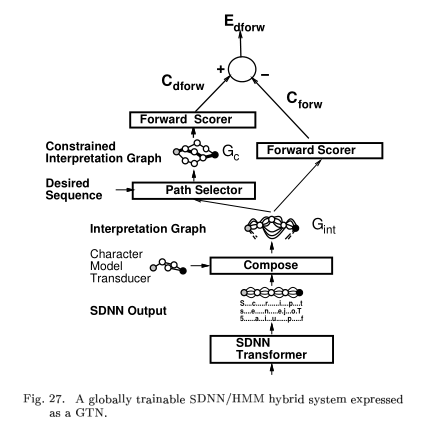
Multiple Object Recognition: Space displacement Neural Network

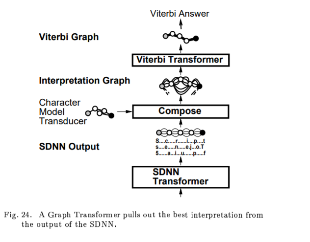
A. Interpreting the Output of an SDNN with a GTN

B.Experiments with SDNN

B.Global Training of  SDNN

 

D.Object Detection and Spotting with SDNN

 

Graph Transformer networks and Transducers

A. previous work

B. Standard Transduction

C. Generalized Transduction

D. Notes on the Graph Structures

E. CTN and Hidden Markov Models

 

An on-line handwriting Recognition system

A.Preprocessing

B.Network architecture

C.Network Training

D. Experimental Results

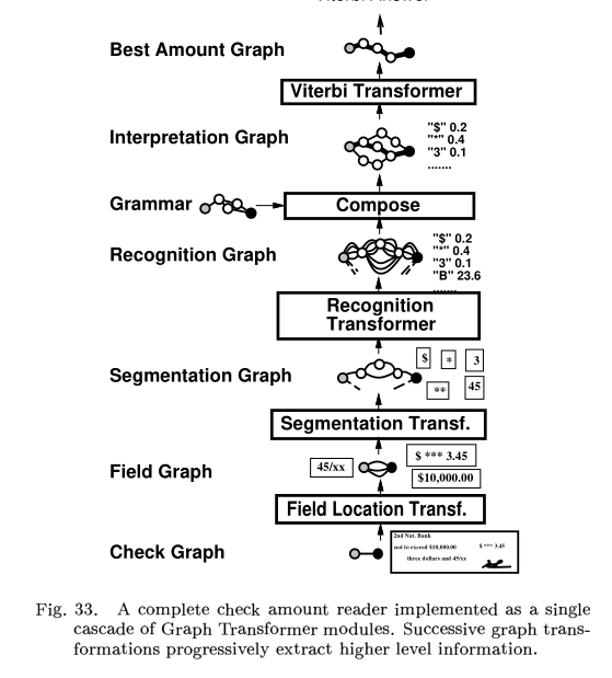
A check reading system

A. A GTN for check Amount Recognition

B. Gradient-Based Learning

C. Rejecting Low Confidence Checks

D. Results

 

APPENDICES

A. Pre-conditions for faster convergence

B. Stochastic Gradient vs Batch Gradient

C. Stochastic Diagonal Levenberg-Marquardt

 

 

 

 

arclab.tistory.com/150

[논문 요약 3] Gradient-Based Learning Applied to Document Recognition