stacking more layer : vanishing/exploding gradients
deeper network : accuracy gets saturated => overfitting 이 아니다.
shortcut connections
identity mappings
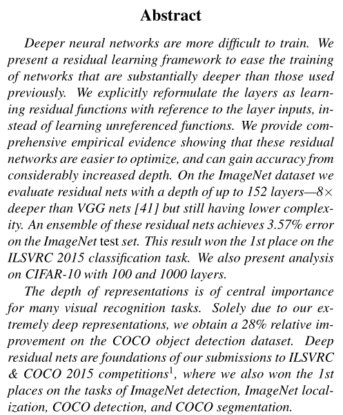
Abstract
neural networks는 깊으면 깊을수록 학습하기 힘들다. 우리는 이전 연구에서 사용된 네트워크들보다 훨씬 학습하기 용이한 residual learning framework 을 제안한다. 여기서 우리는 unreferenced functions을 학습하는 대신, layer의 input을 참조하는 residual function을 명시적으로 재구성한다. 우리가 제공하는 residual networks 는 optimize하기도 쉬우며, 상당히 깊은 네트워크의 경우에도 합리적인 정확도를 얻어낼 수 있음을 실험 결과로 보여준다. ImageNet dataset에서는 VGG nets [41](still having lower complexity ) 보다 8배 깊은 152 layers ResNet을 평가하였다. 이들 residual nets 과 앙상블을 한 결과 ImageNet test set에서 3.57%의 top-5 error를 보였다. the ILSVRC 2015 classification task에서 1등을 하였다. 우리는 CIFAR-10 with 100 and 1000 layers 에서도 분석하였다.
depth of representations는 다양한 visual recognition tasks 에서 매우 중요한 역할을 한다. residual network로부터 얻어낸 deep representation으로부터 COCO object detection dataset에서 28%의 개선 효과를 얻었다. Deep residual network의기초는 ILSVRC & COCO 2015 competitions 에 제출하였다. ImageNet detection/localization, COCO detection/segmentation부문에서 1위를 차지했다.
1. Introduction
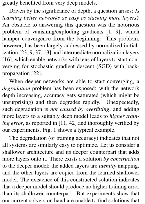
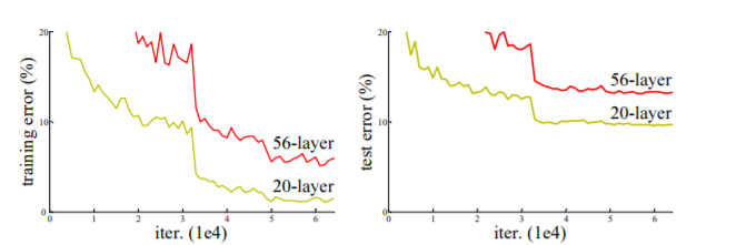
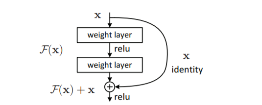
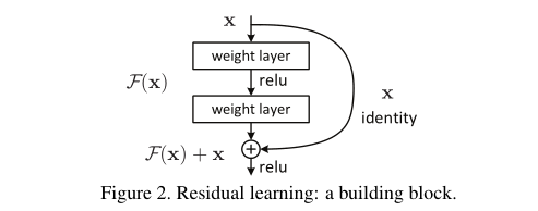
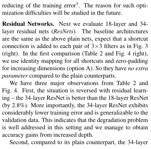
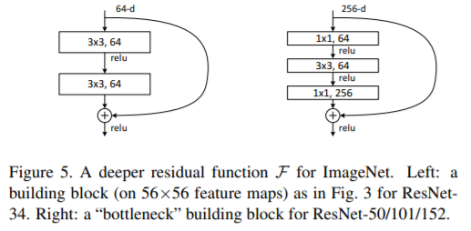
Figure 1. Training error (left) and test error (right) on CIFAR-10 with 20-layer and 56-layer “plain” networks. The deeper network has higher training error, and thus test error. Similar phenomena on ImageNet is presented in Fig. 4.Figure 2. Residual learning: a building block.
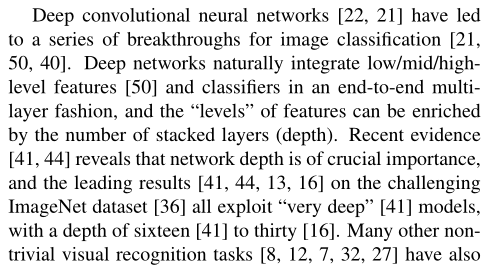
Deep convolutional neural networks [22, 21]의 는 image classification [21, 50, 40]에서 여러가지 돌파구로 이어졌다 . Deep networks 는 low/mid/highlevel features [50]와 classifiers를end-to-end multi-layer fashion으로 자연스럽게 통합하며, 각 features 들의 풍부한 ‘level’은 해당 feature를 추출하기 위해 stacked layer의 depth에 따라 달라진다. 최근의 증거 [41, 44] 따르면 network depth은 결정적 중요하며 , challenging ImageNet dataset [36]의 주요 결과[41, 44, 13, 16]들은 모두 depth가 16[41]~30[16] 정도인 “very deep” [41]을 활용했다. 다른 non-trivial visual recognition [8, 12, 7, 32, 27]에서도 ‘very deep’ model이 큰 도움이 됐다. 깊이의 중요성에 따라 다음과 같은 의문이 생긴다.
더 나은 네트워크를 배우는 것이 stacking more layers 쉬운가? 이 질문에 대한 걸림돌은 처음부터 수렴을 방해하는 vanishing/exploding gradients [1, 9] 의 악명 높은 문제점이 있다. 그러나 이 문제는 주로 normalized initialization [23, 9, 37, 13]와 intermediate normalization layers [16]에 의해 해결되었으며, 이 계층의 수십개의 layers가 있는 network의 back-propagation [22]를 통해 stochastic gradient descent (SGD)에 대한 수렴을 하게 한다.
deeper networks가 수렴하기 시작할 때, 또 다른 성능 저하 문제가 드러난다. 이는 network depth 가 늘어남에 따라
정확도가 포화상태(놀랍지 않을 수 있습니다)에 도달하게 되면 성능이 급격하게 떨어지는 현상을 말한다. 놀랍게도 , 하락문제는 overfitting 때문에 생긴것이 아니라 , depth가 적절히 설계된 모델에 더 많은 layer를 추가하면 training error가 커진다는 이전 연구[11, 42] 결과에 기반한다.아래 Fig.1에서는 간단한 실험을 통해 성능 저하 문제를 보여준다.
예기치 않게, 그러한 저하는 overfitting 에 의해 야기되지 않으며, 적절히 깊은 모델에 더 많은 레이어를 추가하면 [11, 42]에서 보고되고 우리의 실험에서 철저히 검증된 바와 같이 더 높은 ttraining error 로 이어진다. 그림 1은 대표적인 예이다.( Depth 가 깊어질 수록 높은 training error가 높았으며 이에 따른 test error도 높았다. ) 이와 같은 성능 저하(training accuracy의 ) 문제는, 모든 시스템의 최적화 난이도가 쉬운 것은 아님을 나타낸다. shallower architecture와 deeper model를 추가하는 더 깊은 아키텍처를 고려해보자. 이를 만족하는 deeper architecture를 위한 constructed solution이 있긴 하다. added layers 는identity mapping 이며, other layers 는 shallower architecture에서 복사된다. (기존에 학습된 shallower architecture에다가 identity mapping인 layer만 추가하여 deeper architecture를 만드는 방법이다.) 이미 존재한 constructed solution에서 ej deeper model 이 shallower counterpart 보다 더 높은 training error 를 생성해서는 안 된다는 것을 나타낸다. 하지만, 실험을 통해 현재의 solver들은 이 constructed solution이나 그 이상의 성능을 보이는 solution을 찾을 수 없다는 것을 보여준다(or unable to do so in feasible time).
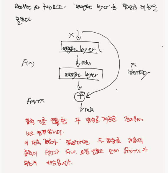
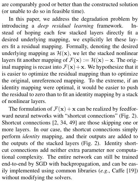
이 논문에서는 우리는 deep residual learning framework을 도입하여 성능 저하 문제를 다룬다. 이 방법은 few stacked layer를 underlying mapping을 직접 학습하지 않고, residual mapping에 맞추어 학습하도록 한다. 공식적으로, 원하는 underlying mappin을 H(x)로 나타낸다면, stacked nonlinear layer의 mapping인 F(x)는 H(x)-x 를 학습하는 것이다. F(x) := H(x)−x 따라서 original mapping은 F(x)+x 로 재구성 된다. 또한, 저자들은 unreferenced mapping인 original mapping보다, residual mapping을 optimize하는 문제가 더 쉽다고 가정한다. 극단적으로 identity mapping 이 optimal일 경우 , nonlinear layers stack에 의한 identity mapping을 맞추는 것보다 residual 0으로 밀어넣는 것이 더 쉬울 것이다. F(x)+x의 공식은 “shortcut connections” 이 있는 feedforward neural networks 으로 구현할 수 있다(Fig. 2). Shortcut connections [2, 34, 49]는 하나 이상의 계층을 건너뛴다. 우리의 예에서는 , shortcut connection은 단순한 identity mapping을 수행하고, 그 출력을 stacked layer의 출력에 더하고 있다(Fig. 2). 이와 같은 identity shortcut connection은 별도의 parameter나 computational complexity가 추가되지 않는다. 전체 네트워크는 여전히backpropagation를 통해 SGD에 의해end-to-end 로 학습이 가능하며, solver 수정 없이도 common library를 사용하여 쉽게 구현할 수 있다 (e.g., Caffe [19]).
우리는 degradation problem를 보여주고 방법을 평가하기 위해 , ImageNet[36]에 대한 comprehensive experiments을 제시한다.
우리는 다음과 같이 보여준다.
1). 우리의 extremely deep residual nets을 최적화하기 쉽지만, 상대적인 “plain” nets (that simply stack layers)은 깊이가 증가할때 더 높은 training error를 나타낸다.
2). deep residual nets는 훨씬 더 깊어진 깊이에서 정확도 향상을 쉽게 누릴 수 있어며 , 이전 네트워크보다 훨씬 향상된 결과를 얻을 수 있다.
CIFAR-10 set[20]에도 유사한 현상이 나타나는데, 이는 우리 방법의 최적화 어려움과 효과가 특정 데이터 세트와만 유사한 것이 아님을 시사한다.우리는 100 이상의 layers를 가진 이 데이터 세트에 대해 성공적으로 훈련된 모델을 제시하고 1000개 이상의 레이어를 가진 모델을 탐색한다.
ImageNet classification dataset [36]에서, 우리는 extremely deep residual nets를 통해 우수한 결과를 얻었다. 우리의 152-layer residual net 는 VGG nets [41]보다 complexity보다 여전히 낮으면서도 ImageNet에 제공된 네트워크 중 가장 깊다. 우리의 ensemble 모델은 ImageNet test set에서 3.57% top-5 error를 기록했으며, ILSVRC 2015 classification competition에서 1등을 차지했다. 또한 extremely deep representations은 other recognition tasks에서 탁월한 성능을 가지고 있으며, ILSVRC & COCO 2015 competitionsImageNet detection, ImageNet localization, COCO detection, and COCO segmentation 부문에서 1등을 차지했다. 이 strong evidence는 residual learning principle이 일반적이라는 것을 보여주며 , 우리는 그것이 다른 시각 및 비전 문제에 적용될 수 있을 것으로 기대한다.
2. Related Work
Residual Representations.
In image recognition에서 VLAD [18]는 dictionary에 대한 residual vectors로 encodes 하는 표현이며, Fisher Vector [30]은 VLAD의 probabilistic version [18] 으로 공식화할 수 있다. 둘 다image retrieval and classification [4, 48] 를 위한 강력하고 얕은 표현이다. vector quantization의 경우, residual vectors [17]를 encoding 하는 것이 original vectors를 encoding하는 것보다 더 효과적이다.
low-level vision 과 computer graphics에서 Partial Differential Equations (PDEs)를 해결하기 위해, 널리 사용되는Multigrid method [3] 은 시스템을 multiple scales에서 subproblems 로 재구성하며, 여기서 각 subproblems 는 a coarser와 a finer scale 사이의 residual solution을 담당한다. Multigrid 의 대안으로는 hierarchical basis pre-conditioning [45, 46]가 있는데 , two scales사이의 residual vectors를 나타내는 변수에 의존한다. [3,45,46] these solvers는 residual nature of the solutions을 인식하지 못하는 standard solvers보다 훨씬 빠르게 수렴하는 것으로 나타났다.
Shortcut Connections.
shortcut connections [2, 34, 49]로 이어지는 Practices and theories은 오래 동안 연구되어 왔다. multi-layer perceptrons(MLPs) 을 학습하는 초기 방법은 네트워크 입력에서 출력[34, 49]으로 연결된 a linear layer를 추가하는 것이다. [44, 24]에서 , a few intermediate layers은 vanishing/exploding gradients를 다루기 위한 auxiliary classifiers에 연결된다. [39, 38, 31, 47]의 논문은 shortcut connections에 의해 구현되는 layer responses, gradients, and propagated errors의 중심을 맞추는 방법을 제안한다. [44]에서 “inception” layer은 a shortcut branch and a few deeper branches로 구성된다.
본 연구와 동시에 , “highway networks” [42, 43]는 gating functions [15]과의 shortcut connections를 제공한다. 이러한 gates는 data-dependent이며 parameter-free our identity shortcuts달리 parameters를 가지고 있다. gated shortcut is “closed” (approaching zero)일 때, highway networks의 layer은 non-residual functions를 나타낸다. 반대로 , 위리의 공식은 항상 residual functions를 학습한다 : 우리의identity shortcuts가 결코 닫히지 않으며, 모든 정보는 항상 전달되며 additional residual functions 를 학습한다. 또한 high-way networks 는 극단적으로 increased depth (e.g., over 100 layers)에도 정확성을 보여주지 않았다.
3. Deep Residual Learning
3.1. Residual Learning
H(x)를 몇 개의 stacked layers(꼭 전체 네트는 아님) 에 의해 적합한 underlying mapping 으로 간주하고, x는 이러한 레이어 중 첫 번째 레이어에 대한 입력을 나타낸다. 만약 multiple nonlinear layers이 complicated functions 2에 점근적으로 근사할 수 있다는 가설이 있다면, H(x) − x (assuming that the input and output are of the same dimensions)와 같은 점근적으로 근사할 수 있다는 가설과 같다. 따라서 stacked layers 이 대략 H(x)일 으로 예상하는 대신, 우리는 이 layers들이 residual function F(x) := H(x) − x에 근접하도록 명시적으로 한다. 따라서 original function는 F(x)+x가 된다. 비록 두 형태 모두 (as hypothesized) 로 원하는 기능을 점근적으로 근사할 수 있어야 하지만, 학습의 용이성은 다를 수 있다.
이 reformulation 는 degradation problem에 대한 counterintuitive phenomena의해 자극을 받는다(Fig. 1, left). introduction에서 논의 한것과 같이 , added layers이 identity mappings으로 구성될 수 있다면, deeper model 은 shallower counter-part보다 training error를 가져야 한다. degradation problem는 solvers 가 여러 nonlinear layers에 의한 identity mappings을 근사화하는데 어려움이 있을 수 있음을 시사한다.residual learning을 통해 , identity mappings이 최적인 경우, solvers 는 단순히 identity mappings에 접근하기 위해 multiple nonlinear layers weights 를 0으로 유도할 수 있다.
실제의 경우, identity mappings이 최적일 가능성이 낮지만, 우리의 reformulation은 문제를 precondition 하는 데 도움이 될 수 있다. optimal function가 zero mapping보다 identity mapping이 더 가까울 경우, solver 는 새로우 기능으로 함수를 학습하는 것보다identity mapping을 참조하여 perturbations 을 찾는 것이 더 쉬워야 한다.
실험에서는 학습된 residual function에서 일반적으로 작은 반응이 있다는 결과를 보여준다(Fig.7 참조). 이 결과는 identity mapping이 합리적인 preconditioning을 제공한다는 것을 시사한다. 우리는 실험(Fig.7)을 통해 , 학습된residual functions가 일반적으로 작은 반응을 가지고 있다는 것을 보여주며,identity mappings이 합리적인 preconditioning을 제공한다는 것을 시사한다.
3.2. Identity Mapping by Shortcuts
우리는 모든 few stacked layers마다 residual learning을 사용한다. building block은 Fig.2에서 나와있다. 공식적으로 , 이 논문에서는 우리는 a bulding block 을 아래와 같이 정의했다.
y = F(x,{W i }) + x. (1)
x와 y는 각각 building block의 input와 output vector이다.
function F(x,{W_i })는 학습 해야 할 residual mapping이다.
Fig. 2 에서 two layers가 있는 예를 들면, F = W_2 σ(W_1 x)로 나타낼 수 있다.
여기서 σ는 ReLU [29]를 나타내며 간소화를 위해 biases 는 생략되었다.
F + x연산은 shortcut connection 및 element-wise addition으로 수행된다. addition 후에는 second nonlinearity로 ReLU를 적용한다. (i.e., σ(y), see Fig. 2)
Eqn.(1) 의 shortcut connection 연산은 별도의 parameter나 computational complexity가 추가되지 않는다. 이는 실제로 매력적일 뿐만 아니라plain network와 residual network 간의 를 비교하는 데에도 중요하다.(공정한 비교를 가능하게 해준다. ) 우리는 parameters의 수, depth, width, 및 computational cost(except for the negligible element-wise addition-> element-wise addition은 무시할 정도이다. ) 동일한 plain/residual networks를 공정하게 비교할 수 있다.
Eqn.(1)에서 x와 F의 dimensin이 같아야 한다. 그렇지 않은 경우 (예: 입력/출력 채널을 변경할 때), shortcut connections을 통해 a linear projection W_s 를 수행하여 dimensions maching시킬 수 있다.
y = F(x,{W i }) + W s x. (2)
Eqn.(1)에서 square matrix W_s를 사용할 수 있다. 하지만 우리는 실험을 통해 identity mapping이 degradation problem를 해결하기에 충분하고 경제적이므로 W_s는 dimensions maching 시킬 때만 사용하는 것을 보여줄 수 있다.
residual function F 의 형태는 유연하게 결정할 수 있다. 즉, 본문에서는 two or three layers (Fig. 5)가 function F를 사용하지만, 더 많은 layer를 포함하는 것도 가능하다. 하지만,F가 단 하나의 layer만 갖는 경우에는 Eqn.(1)은 단순 linear layer와 유사하다. y = W_1 x+x 이 layer에서는 이점을 관찰하지 못했다.
우리는 또한 위의 수식이 단순성을 위해fully-connected layers에 대한 것이지만, convolutional layers에 적용할 수 있다는 점에 주목한다. function F(x,{W_i })는 multiple convolutional layers를 나타낼 수 있다 . element-wise addition는 channel by channel(channel 별)로 two feature maps에서 수행된다.
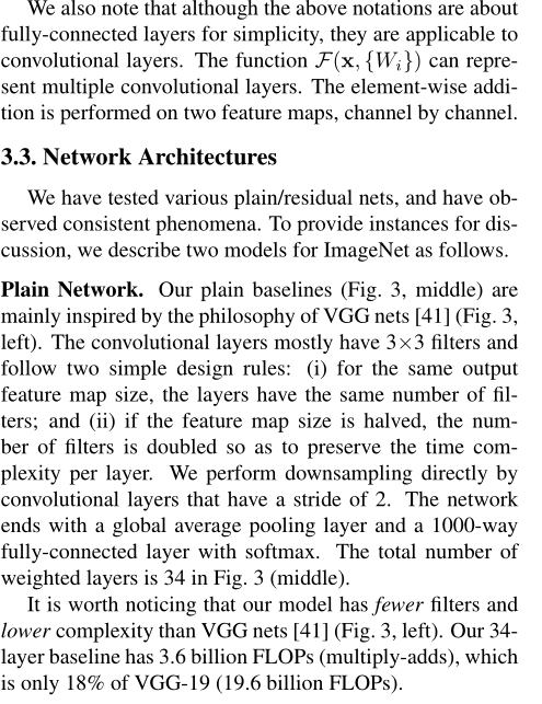
3.3. Network Architectures
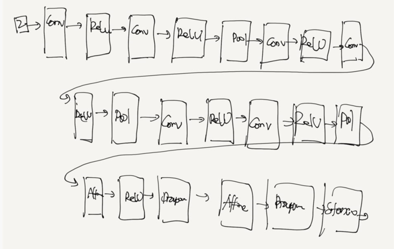
이 논문에서는 다양한 형태의 plain/residual network에 대해 테스트 했으며, 일관된 현상을 관찰한다. instances for discussion을 증명하기 위하여 , 우리는 ImageNet dataset을 위한 두 모델을 다음과 같이 정의했다.
Plain network
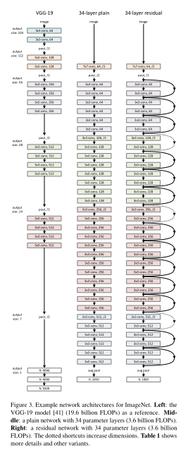
우리의 plain의 baseline(Fig.3 middle)은 주로 VGG net(Fig.3 left)의 철학에서 영감을 받았다. convolutional layers는 대부분 3x3 filter를 가지며, 다음과 같이 두 가지의 간단한 규칙에 따라 디자인 된다.
1). 동일한 output feature map size에 대해, layer의 filters수는 동일하다.
2). feature map size가 절반으로 줄어들 경우, layer 당 time complexity를 보전하기 위해 filter의 수를 2배로 한다.
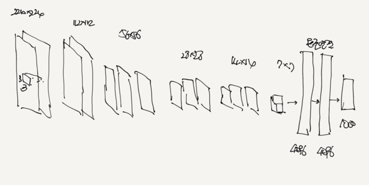
stride 2인 convolutional layers에 의해 직접 downsampling을 사용했다. 네트워크의 마지막에는 global average pooling layer 와 activation이 softmax인 1000-way fully-connected laye로 구성된다 . Fig. 3 (middle)에서 총 weighted layers 수는 34이다. 우리의 모델은VGG nets [41] (Fig. 3, left)보다 filter수가 작고 complexity 가 lower 다는 것을 주목할 필요가 있다. 우리의 34개의 layer로 구성된 이 baseline plain network(Fig.3 가운데)는 3.6 billion FLOPs이며, 이는 VGG-19(19.6 billion FLOPs)의 18%에 불과하다.
Residual network
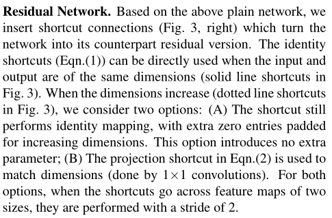
위의 plain network의 가반으로, 우리는 shortcut connections((Fig. 3, right) 을 삽입하여 residual version의 network를 만든다. (Fig.3 오른쪽) identity shortcut(Eqn.1)은 input과 output이 동일한 dimension인 경우(Fig.3의 solid line shortcuts)에는 직접 사용할 수 있다.
dimension이 증가하는 경우(Fig.3의 dotted line shortcuts)에는 아래의 두 옵션을 고려한다.
(A) shortcut 는 여전히 identity mapping을 수행하며,
zero entry padding 를 추가되어서 dimensions을 널린다. 이 옵션은 별도의 parameter가 추가되지 않음
(B) Eqn.2의 projection shortcut을 dimension matching에 사용한다. (done by 1x1 convolutions). shortcut connection이 다른 크기의 feature map 간에 mapping될 경우, 두 옵션 모두 strides를 2로 수행한다.
y = F(x,{W i }) + W s x. (2)
FLOPS :플롭스는 컴퓨터의 성능을 수치로 나타낼 때 주로 사용되는 단위이다.
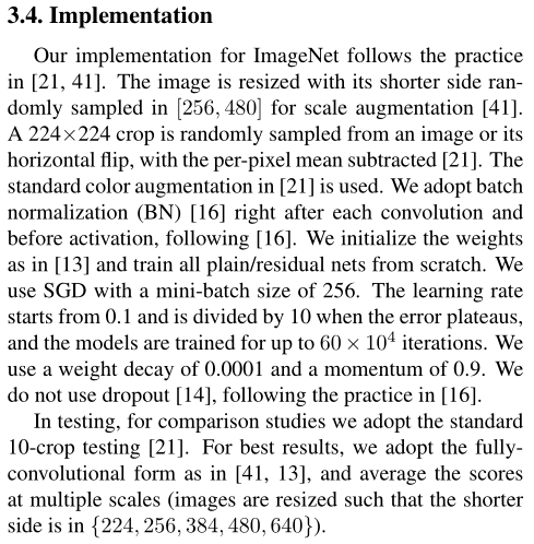
3.4. Implementation
논문에서 ImageNet dataset에 대한 실험은 [21, 41] 방법에 따른다. 이미지는 scale augmentation [41]를 위해 [256, 480]에서 무작위하게 샘플링 된 shorter side를 사용하여 rescaling된다. 224x224 crop은 horizontal flip with per-pixel mean subtracted [21] 이미지 또는 이미지에 무작위로 샘플링 된다. standard color augmentation in [21] 도 사용된다. 우리는 [16]에 이어 , 각 convolution 직후와 activation 전에 batch normalization (BN) [16]를 사용했다. [13] 과 같이 weights 를 초기화하고 모든 plain/residual nets를 처음부터 학습한다. 우리는 SGD 사용하고 mini-batch size는 256이다. learning rate는 0.1에서 시작하여, error plateau 나올때 rate를 10으로 나누어 적용하며, 모델은 최대 iteration은 6X10^4회이다. 우리는 weight decay는 0.0001, momentum은 0.9로 한 SGD를 사용했다.[16]의 관례에 따라 dropout[14]을 사용하지 않는다.
테스트에서 , 비교 연구를 위해 , standard 10-crop testing [21]를 채택한다.
최상의 결과를 위해 , 우리는 [41, 13] 와 같은 fully convolutional form 적용하였으며 , multiple scales를 평균화하였다 (images are resized such that the shorter side is in {224, 256, 384, 480, 640}).multiple scale은 shorter side가 {224, 256, 384, 480, 640}인 것으로 rescaling하여 사용한다.
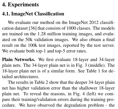
4. Experiments
4.1. ImageNet Classification
우리는 1000 classes로 구성된 ImageNet 2012 classification dataset[36] 에서 제안하는 방법을 평가한다.
모델의 학습및 테스트 에 사용된 데이터는 아래와 같다.
training images : 1.28 million
validation images : 50k
test images images : 100k => final result
테스트 결과는 top-1 error와 top-5 error를 모두 평가한다.
Plain Networks
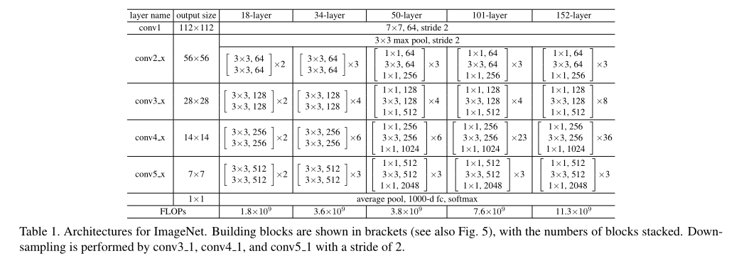
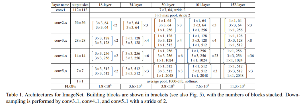
우선 우리는 18-layer and 34-layer plain nets에 대해서 평가한다. 34-layer plain net은 Fig. 3 (middle)에 있다. 18-layer plain net 는 비슷한 형태로 구성된다 . 상세한 구조는 Table 1에서 보여준다.
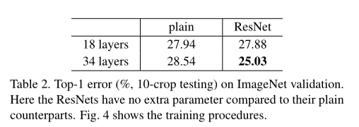
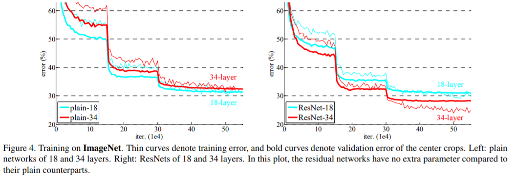
plain net = > Table 2 의 결과에서는 18-layer plain net 에 비해, deeper 34-layer plain net 의 validation error가 높다는 것이다. => deeper 34-layer plain net의 validation error가 높다 .
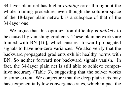
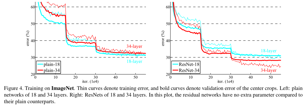
이유를 알아보기 위 Fig. 4 (left)에서 우리는 학습 중의 training/validation error를 비교한다. 우리는 degradation problem 를 관찰했다. - 18-layer plain network의 solution space는 34-layer plain network의 subspace임에도 불구하고, 오히려 34-layer plain net 인 경우 학습 과정 전반에서 더 높은 training error 를 갖는다.
논문의 저자들은 여기서 직면하는 optimization difficulty가 vanishing gradients에 의한 것과 같지 않다고 하였다. 그 이유는 plian network 가 BN [16]을 포함하여 학습하기 때문에 forward propagated signal의 분산이 0이 아니도록 보장한다. 우리는 또한 backward propagated gradients가 BN과 함께healty norm을 보이는 것도 확인했기 때문이다. 따라서forward/backward signal은 vanishing 하지 않았다고 볼 수 있다. 실제로 , Table 3 의 결과를 따르면 34-layer plain network가 여전히 경쟁력 있는 정확도를 달성했으며, 이는 solver의 작동이 이루어지긴 한다는 것을 의미한다. 저자들은 또한, deep plain network는 exponentially low convergence rate를 가지며, 이것이 training error의 감소에 영향 끼쳤을거라 추측하고 있다. optimization difficulties의 원인에 대해서는 미래에 배울 것이다.
=> 층이 깊을 수록 training error가 낮은 것 보다 낮다. optimization difficulties가 gradient vanishing 문제가 아닌것 같고 exponentially low convergence rate를 가지고 있으서 training error의 감소에 영향 끼쳤을거라 추측하고 있다.
We have experimented with more training iterations (3×) and still observed the degradation problem, suggesting that this problem cannot be feasibly addressed by simply using more iterations. => 저자들은 더 많은training iterations (3×) 으로 실험했지만 여전히degradation problem를 관찰하였으며 , 이는 단순히 더 많은 반복을 사용하는 것으로 이 문제를 해결할 수 없음을 시사한다.
Residual Networks
다음으로 18-layer 및 34-layer residual network(이하 ResNet)를 평가한다.baseline architecture는 위의 plain network와 동일하며, Fig.3의 오른쪽과 같이 각 3x3 filter pair에 shortcut connection을 추가했다. In the first comparison (Table 2 and Fig. 4 right), 모든 shortcut connection은 identity mapping을 사용하며, dimension matchings (option A)을 위해서는 zero-padding을 사용한다(3.3절의옵션 1참조). 따라서, 대응되는 plain network에 비해 추가되는 parameter가 없다.
Table.2와 Fig.4에서 알 수 있는 3가지 주요 관찰 결과는 다음과 같다.
1. residual learning으로 인해 상황이 바뀌었다. 34-layer ResNet이 18-layer ResNet(by 2.8%)보다 우수한 성능을 보인다. 또한, 34-layer ResNet이 상당히 낮은 training error를 보였으며, 이에 따라 향상된 validation 성능이 관측됐다. 이는 성능 저하 문제가 잘 해결됐다는 것과, 증가된 depth에서도 합리적인 accuracy를 얻을 수 있다는 것을 나타낸다.
2. 34-layer ResNet은 이에 대응하는 plain network와 비교할 때, validation data에 대한 top-1 error를 3.5% 줄였다(Table.2 참조). 성공하게 training errors을 줄이는 것은 (Fig. 4 right vs. left) 결곽 있다. 이는 extremely deep systems에서 residual learning의 유효성을 입증하는 결과다.
3. 마지막으로는 , 18-layer plain/residual network 간의 정확도(Table 2) 유사한 성능을 보였지만, Fig.4에 따르면 18-layer ResNet이 더욱 빠르게 수렴한다r (Fig. 4 right vs. left). 이는 network가 “not overly deep”한 경우(18-layers의 경우), 현재의 SGD solver는 여전히 plain net에서도 좋은 solution을 찾을 수 있다는 것으로 볼 수 있다. 하지만, 이러한 경우에도 ResNet에서는 빠른 수렴속도를 기대할 수 있다.
Identity vs. Projection Shortcuts
앞에서 parameter-free한 identity shortcut이 학습에 도움 된다는 것을 보였다. 이번에는 Eqn.2의 projection shortcut에 대해 조사하자. Table.3에서는 다음 3가지 옵션에 대한 결과를 보여준다.
zero-padding shortcut는 dimension matching에 사용되며, 모든 shortcut는 parameter-free하다(Table.2 및 Fig.4의 결과 비교에 사용됨).
projection shortcut는 dimension을 늘릴 때만 사용되며, 다른 shortcut은 모두 identity다.
모든 shortcut은 projection이다.
Table.3에서는 3가지 옵션 모두 plain network보다 훨씬 우수함을 보여준다. 우리는 이것이 A의 zero-padded dimensions이 실제로 esidual learning이 없기 때문이라고 주장한다. C에 비해서 B보다 약간 낫고 , 우리는 이것을 많은 (thirteen) projection shortcuts에 의해 도입된 추가 parameters 때문이라고 본다. 그러나 A/B/C 간의 작은 차이는 projection shortcuts가 degradation problem를 해결하는데 필수적이지 않다는 것을 나타냅니다. 따라머 memory/time complexity와 model size를 줄이기 위해 이 논문의 나머지 부분에서는 옵션 C를 사용하지 않느다. Identity shortcuts은 아래에 소개된 bottleneck architecture의 complexity를 증가시키지 않는데 특히 중요하다.
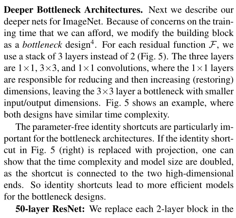
Deeper Bottleneck Architectures.
다음으로 mageNet을 위한deeper nets에 대해 설명한다. 학습 시간에 대한 우려로 인해 building block as a bottleneck desig으로 설계한다.
Deeper non-bottleneck ResNets (e.g., Fig. 5 left) also gain accuracy from increased depth (as shown on CIFAR-10), but are not as economical as the bottleneck ResNets. So the usage of bottleneck designs is mainly due to practical considerations. We further note that the degradation problem of plain nets is also witnessed for the bottleneck designs. =>Deeper non-bottleneck ResNets (예: Fig. 5 lef ) 도 증가된 depth (CIFAR-10에 표시된 대로)에서 정롹도를 얻지만 bottleneck ResNets만큼 경제적이지는 않는다. 그래서 bottleneck designs의 사용은 주로 실용적인 고려 사항 때문이다. 우리는 또한 bottleneck designs에서도 plain nets의 degradation problem 가 목격된다는 것을 주목한다.
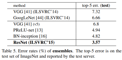
각 residual function F 에 대해, 우리는 2 layers 대신 3 layers의 stack을 사용한다(Fig.5 참조). three layers는 1×1, 3×3, and 1×1 convolutions이며 , 여기서
1×1 layers는 (restoring) dimensions 크기 를 을 줄이거나 증가시키는 용도로 사용하며 ,
3×3 layer의 input/output의 dimentsion을 줄인 bottleneck 으로 둔다. Fig.5에서는 2-layer stack과 3-layer stack가 유사한 디자인과 유사한 time complexity을 갖는 예를 보여준다 . 둘은 유사한 time complexity를 갖는다.
여기서 parameter-free는 identity shortcuts는 bottleneck architectures에서 특히 중요하다. 만약 Fig. 5 (right) 의 identity shortcut가 projection으로 대체된다면, shortcut이 두 개의 high-dimensional 출력과 연결되므로 time complexity와 model size가 두 배로 늘어난다. 따라서 identity shortcut은 이 bottleneck design을 보다 효율적인 모델로 만들어준다.
50-layer ResNet:
우리는 34-layer ResNet의 2-layer block들을 3-layer bottleneck block으로 대체하여 50-layer ResNet(Table 1)을 구성했다. 우리는 크기를 늘리기 위해 option B 를 사용한다. 이 모델은 3.8 billion FLOPs 를 가지고 있다.
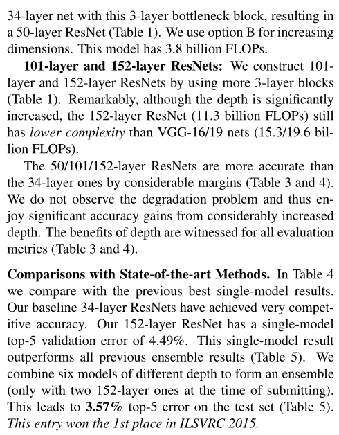
101-layer and 152-layer ResNets: 우리는 더 많은 3-layer bottleneck block을 사용하여 101-layer 및 152-layer ResNet을 (Table 1) 구성했다. depth가 상당히 증가했음에도 상당히 높은 정확도가 결과로 나왔다. 152-layer ResNet (11.3 billion FLOPs)은 VGG-16/19 nets (15.3/19.6 billion FLOPs)보다 복잡성이 낮다.
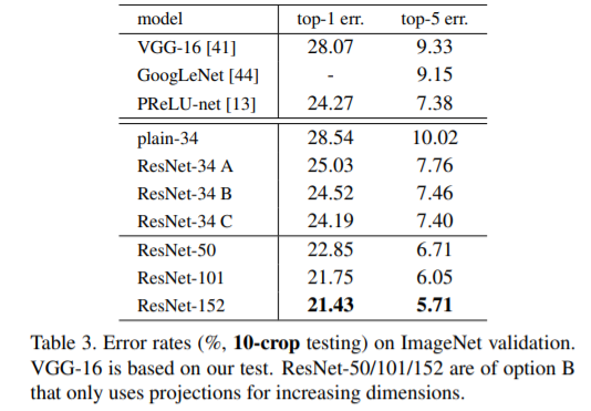
50/101/152-layer ResNets는 34-layer ResNets 보다 상당한 margins 으로 정확하다 (Table 3 and 4).
Comparisons with State-of-the-art Methods
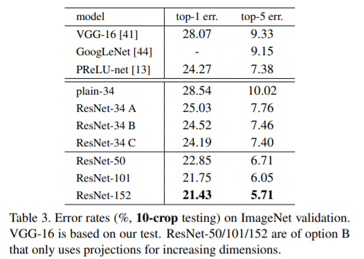
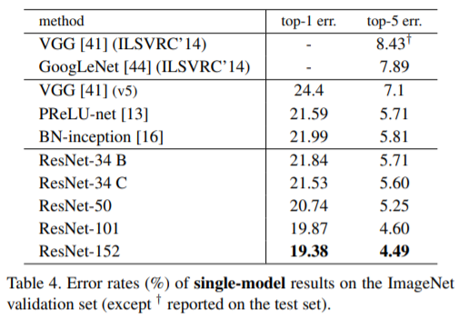
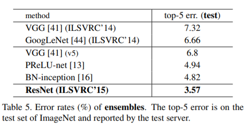
Table.4에서는 previous best single-model 결과와 비교한다. 우리의 baseline인 34-layer ResNet은 previous best에 비준하는 정확도를 달성했다. 152-layer ResNet의 single-model top-5 error는 4.49%를 달성했다. 이 single-model result 결과는 이전의 모든 ensemble result를 능가하는 성능이다(Table.5 참조). 또한, 우리는 서로 다른 depth의 ResNet을 6개 모델을 (ensemble)을 형성한다. (submitting시 152-layer 모델 2개만 있음)이로 하여 tes set에서 top-5 test error를 3.57%까지 달성했다(Table 5). 이는 ILSVRC 2015 classification task에서 1위를 차지했다.
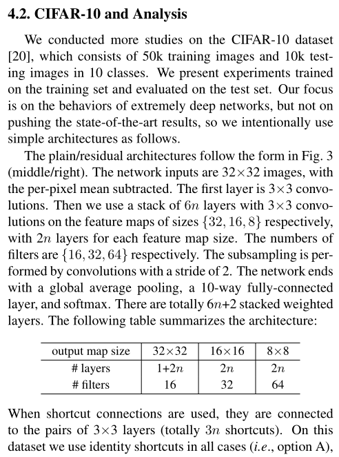
4.2. CIFAR-10 and Analysis
논문에서는 CIFAR-10 dataset[20]에 대한 더 많은 연구를 수행했다.
CIFAR-10 dataset :
10개의 classes
training images가 50 k
testing images 10k
우리는 training set에서 학습되고 test set에서 평가된 실험을 제시한다. 우리는 extremely deep networks의 동작에 초점을 맞추고 있지만 state-of-the-art results를 추진하는 데는 초점을 맞추지 않기 때문에 의도적으로 다음과 같은 간단한 architecture를 사용했다.
plain/residual architectures는 Fig. 3 (middle/right)의 양식을 따른다.
network의 input은 per-pixel mean subtracted 32x32 이미지이다.
첫 번째 layer는 3x3 cconvolutions이다.그런 다음 sizes {32, 16, 8} respectively feature maps 에서 각각3×3 convolutions을 가진 stack of 6n layers를 사용하고 각 feature map size에 대해 2n layers를 사용한다. filters 수는 각각 {16, 32, 64}개이다. 그 subsampling 은 stride 2으로 convolutions 을 수행된다. network의 ends는 global average pooling, a 10-way fully-connected layer, and softmax로 구성된다. 총 6n+2 stacked weighted layers가 있다. 다음 표는 아키텍처가 요약되어 있다.
shortcut connections가 사용될 때 , 3×3 layers 쌍 (totally 3n shortcuts) 에 연결된다. 이 dataset에서 우리는 모든 경우(즉 option A) 에 identity shortcuts를 사용하므로 우리의 residual models은 plain counterparts와 정확히 동일한 depth, width, and number of parameters수를 갖는다.
학습 진행 방법은 다음과 같다.
weight decay : 0.0001
momentum : 0.9
weight initialization in [13] and BN [16]수렴하고 but with no dropout.
4개의 pixel이 각 side에 padded 있으며 32×32 crop이 padded 된 이미지 또는 horizontal flip에서 무작위로 샘플링된다.
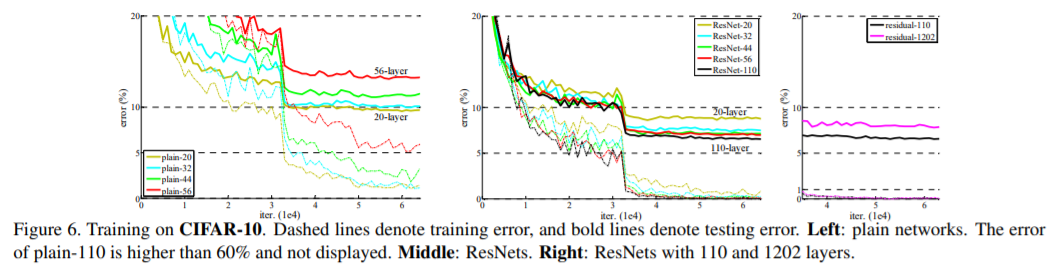
테스트를 위하여 우리는 original 32×32 image의 single view만 평가한다. 우리는n = {3, 5, 7, 9}에서는 20, 32, 44, and 56-layer networks를 비교한다. Fig. 6 (left)은 plain network의 결과를 보여준다. deep plain nets 은 depth가 증가하여 , going deeper수록 training error 가 커진다. 이 현상은 ImageNet (Fig. 4, left) 및 MNIST (see [42])의 현상과 유사하며 , 이는 이러한 최적화 어려움이 근본적인 문제임을 시사한다.
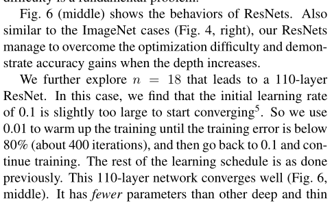
Fig. 6 (middle) 는 ResNets의 학습 결과를 보여준다. 또한 ImageNet cases (Fig. 4, right)와 유사하게 ResNets은 optimization 어려움을 극복하고 깊이가 커질 때 정확도가 향상됨을 입증한다.
110-layer ResNet으로 이어지는 n = 18에 대해서 자세히 살펴본다. 이 경우initial learning rate가 0.1인 것이 수렴을 시작하기에는 약간 너무 크다는 것을 알 수 있다.
With an initial learning rate of 0.1, it starts converging (<90% error) after several epochs, but still reaches similar accuracy. => initial learning rate of 0.1으로 , 몇 epoches후 수렴(<90% error)을 시작하지만 여전히 유사한 정확도에 도달한다.
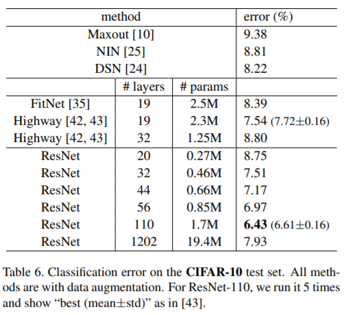
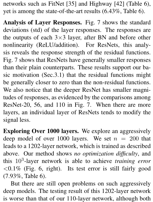
따라서 0.01을 사용하고 training error가 80% (약 400 iterations)미만으로 떨어질 때까지 학습 warm up을 수행한 다음 0.1로 다시 돌아가서 학습을 계속 한다. 나머지 learning schedule은 이전과 같다. 110-layer network 는 잘 수렴된다(Fig. 6, middle). FitNet [35] 및 Highway [42](Table 6)와 같은 다른 deep and thin networks 보다 parameters가 적지만 state-of-the-art results (6.43%, Table 6)을 달성했다 .
Analysis of Layer Responses.
Analysis of Layer Responses.
Fig.7은 layer response의 std(standard deviation)를 보여준다. response는 BN 이후와 다른 nonlinearity(ReLU/addition) 이전의 각 3x3 conv layer의 output이다. ResNets의 경우, 이 분서을 통해 residual functions의 response strength 를 확인할 수 있다. Fig.7에서는 ResNet이 일반적으로 plain counterparts보다 반응이 적다는 것을 보여준다. 이러한 결과는 residual function이 non-residual function보다 0에 가까울 수 있다는 우리의 basic motivation (Sec.3.1)를 뒷받침한다. 우리는 또한 Fig.7의 ResNet-20, 56 및 110 사이의 비교에서 증명된 바와 같이 더 깊은 ResNet의 Response가 더 작다는 것을 알 수 있다. layers가 많을 수록 ResNets 의 개별 layer은 신호를 덜 수정하는 경향이 있다.
Exploring Over 1000 layers.
우리는 100개 이상의 layer로 구성된
aggressively deep model을 탐구한다. 위에서 설명한 대로 학습되는 1202-layer network로 이어지는 n = 200을 설정한다. 우리의 방법은 optimization 어려움이 없으며, 이 103-layer network 는 training error <0.1% (Fig. 6, right). test error는 여전히 상당히 양호한 결과를 보였다. (7.93%, Table 6)
그러나 그러한 aggressively deep models에 대해서는 아직 해결되지 않은 문제들이 있다. 1202-layer network의 test 결과는 110-layer ResNet의 test결과보다 더 나쁘다. 우리는 이것이 과적합 때문이라고 주장한다. 1202-layer network는 CIFAR-10 작은 dataset에 test용으로 불필요하게 클 수 있다. (19.4M) maxout [10] 또는 dropout [14]와 같은 강력한 regularization 를 적용하여 이 dataset에 대한 최상의 결과([10, 25, 24, 35]) 를 얻는다. 이 논문에서 우리는 maxout/dropout을 사용하지 않고,optimization의 어려움에 집중하는 것을 방해하지 않고 설계상 deep and thin architectures를 통해 regularization 만 시행한다. 하지만 더 강력한
regularization 와 결합하면 결과가 향성될 수 있는데, 앞으로 우리가 연구할 것이다.
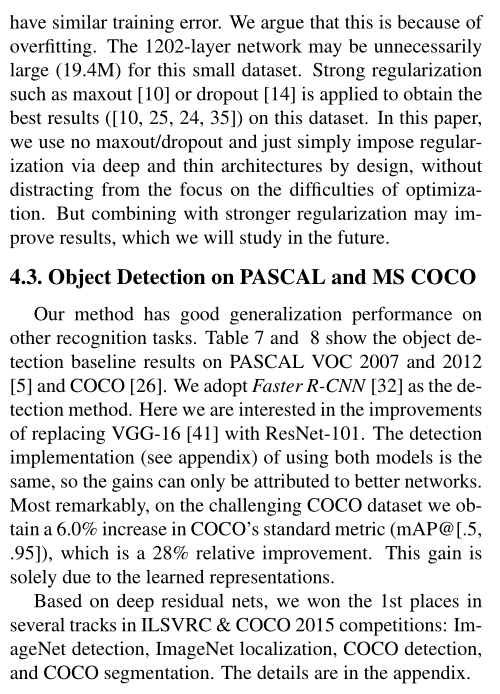
4.3. Object Detection on PASCAL and MS COCO
우리의 방법은 다른 recognition tasks에서 좋은 generalization performance 가지고 있다.
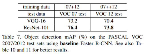
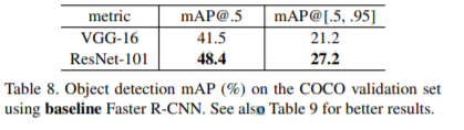
Table 7 and 8에는 PASCAL VOC 2007 and 2012 [5] and COCO [26]의 object detection baseline results가 표시된다. detection method으로 Faster R-CNN [32]을 채택한다. 여기서는 VGG-16 [41] with ResNet-101로 교체하는 개선 사항에 대해 살펴봅시다. 두 모델을 사용하는 detection implementation (see appendix) 은 동일하므로 이득은 더 나은 networks에만 얻을 수 있다. 가장 주목할 만한 점은 까다로운 COCO 데이터 세트에서 COCO 의 standard metric (mAP@[.5,.95])이 6.0%증가하여 상대적으로 28% 향상되었다. 이 이득은 오로지 학습된 표현에 기인한다.
deep residual nets 기반으로 , ILSVRC & COCO 2015 competitions에서 , 여러 tracks에서 1위를 차지 했다: ImageNet detection, ImageNet localization, COCO detection, and COCO segmentation. 자세한 내용은 appendix에 있다.
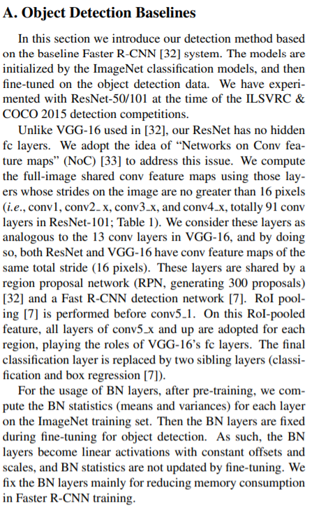
A. Object Detection Baselines
이 section에서는 baseline Faster R-CNN [32] 시스템을 기반으로 detection method을 소개한다. 모델은 ImageNet classification models에 의해 초기화된 다음 bject detection data에서 fine-tuned 된다. 우리는 ILSVRC & COCO 2015 detection competitions 당시 ResNet-50/101으로 실험했다.
[32]에서 사용 되는 VGG-16과 달리 ResNet에는 hidden fc layers이 없다 . 우리는이 문제를 해결하기 위해“Networks on Conv feature maps”(NoC) [33]라는 아이디어를 채택했다. 이미지에 대한 strides 이 16 pixels (i.e., conv1, conv2 x, conv3 x, and conv4 x, totally 91 conv layers in ResNet-101; Table 1)를 사용하여 전체 이미지 shared conv feature maps을 계산한다. 우리는 이러한 레이어가 VGG-16의 13 개 conv 레이어와 유사하다고 간주하며, 그렇게 함으로써 ResNet과 VGG-16은 모두 동일한 총 stide (16 pixels) conv feature maps을 갖게 된다. 이러한 layer은 egion proposal network (RPN, generating 300 proposals) [32]와 Fast R-CNN detection network [7]에 의해 공유된다. RoI pooling [7] 은 conv5-1 이전에 수행된다. 이 RoI-pooled feature에서는 VGG-16’s fc layers역할을 수행하는 모든 conv5 x 이상의 계층이 각 지역에 채택된다. 마지막 classification layer은 두개의 sibling layers (classification and box regression [7])으로 대체된다.
BN layer를 사용하기 위해 pre-training 후 ImageNet training set에서 각 layer에 대한 BN statistics(means and variances)를 계산한다. 그런 다음 object detectoin를 위한 fine-tuning 에 BN layer가 고정된다. 따라서 BN layer는 일정한 offsets and scales로 linear activations 가 되며 , BN statistics 은 fine-tuning 할때 업데이터되지 하지 않는다. 우리는 주로 Faster R-CNN training에서 메모리 소비를 줄이기 위해 BN layer를 고정한다.
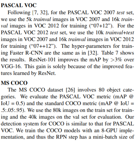
PASCAL VOC
[7, 32]에 따라 ASCAL VOC 2007 test set의 경우 , VOC 2007의 5k trainval 이미지와 VOC 2012의 16k trainval 이미지를 학습에 사용한다(“07+12”). PASCAL VOC 2012 test set의 경우, VOC 2007의 10k trainval+test images와 VOC 2012의 16k trainval images를 학습에 사용한다. Faster R-CNN 학습을 위한 hyper-parameters는 [32]와 동일하다. Table 7은 결과를 보여준다. ResNet-101 은 VGG-16에 비해 mAP를 3% 이상 향상시켰다. 러한 이점은 전적으로 ResNet에서 학습한 향상된 기능 때문이다.
MS COCO
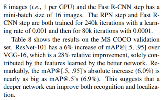
MS COCO dataset [26]는 80개의 object categories로 포함한다. PASCAL VOC metric (mAP @IoU = 0.5)과 standard COCO metric (mAP @ IoU =.5:.05:.95)을 평가한다. 학습을 위해 train set의 80k 이미지를 사용하고 평가를 위해 val set 의 40k를 사용한다. 우리의 detection system은 PASCAL VOC와 유사하다. 우리는 8-GPU implementation으로 COCO 모델을 교육하므로 RPN단계는 8 images (i.e., 1 per GPU) 의 mini-batch size를 가지며 Fast R-CNN step은 16 images mini-batch size를 갖는다. RPN step 와 Fast RCNN step는 모두 learning rate가 0.001인 240k iterations 과 0.0001인 80k iterations 에 대해 훈련 된다.
Table 8 은 MS COCO validation set의 결과를 보여준다. ResNet-101은 VGG-16에 비해 mAP@[.5, .95]가 6% 증가했으며, 이는 더 나은 네트워크에 의해 학습된 기능에 대해서만 28%의 상대적 개선이다. 놀랍게도, mAP@[.5,.95]의 absolute increase (6.0%)은 mAP@.5’s (6.9%)와 거의 같다. 이것은 network가 더 깊어질수록 ecognition and localization과 모두 향상될 수 있음을 시사한다.
B. Object Detection Improvements
completeness를 위해 competitions 개선사항을 보고 드린다. 이러한 개선 사항은 deep features을 기반으로 하므로 residual learning에서 이득을 얻을 수 있다.
MS COCO
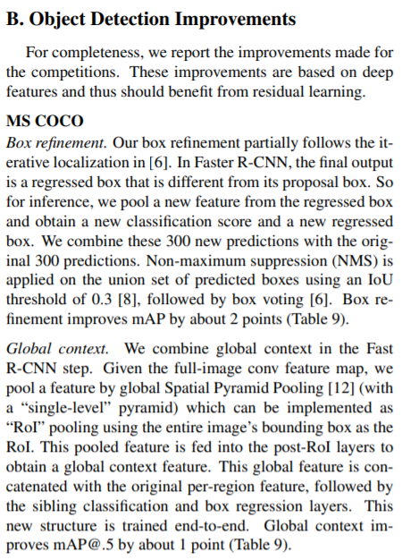
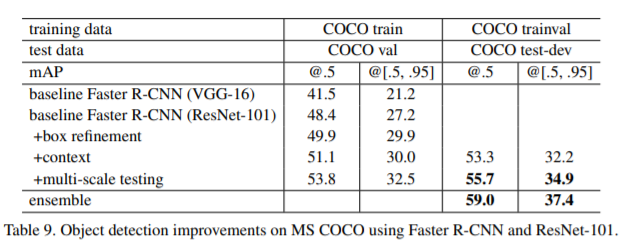
Box refinement. box refinement은 부분적으로 [6]의 iterative localization 파악을 따른다. Faster R-CNN에서 final output은 proposal box와 다른 regressed box이다. 그래서 추론을 위해, 우리는 regressed box 에서 새로운 기능을 pool 하고 새로운 classification score와 새로운 regressed box를 얻는다. 우리는 이 300 new predictions 과 original 300 predictions을 결합한다. Non-maximum suppression (NMS)는 0.3 [8]의 IoU threshold을 사용한 다음 box voting [6]를 사용하여 predicted boxes의 union set에 적용된다. Box refinement 는 mAP 를 2 points (Table 9) 개선한다.
Global context. Fast R-CNN step에서 global context를 결합한다. full-image conv feature map이 주어지면 전체 이미지의 bounding box를 ROI로 사용하여 “RoI” pooling으로 구현할 수 있는 global Spatial Pyramid Pooling [12] (with a “single-level” pyramid) 에 의해 feature를 pooling한다. 이 pooled feature 은 global context feature을 얻기 위해 post-RoI layers 에 공급된다. 이 global feature는 original per-region feature와 연결된 다음 sibling classification and box regression layers 과 연결된다. 이 new structure는end-to-end로 학습된다. Global context는 mAP@.5를 약 1 point (Table 9)향상시킨다.
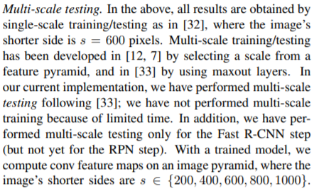
Multi-scale testing. 위에서 모든 결과는 [32]와 같이 single-scale training/testing을 통해 얻을 수 있으며, 여기서 영상의 더 짧은 면은 s = 600pixels입니다. Multi-scale training/testing 는 feature pyramid에서 scale 을 선택하여 [12, 7]에서 개발되었으며 [33] 에서는 maxout layers를 사용하여 개발되었다. 현재 구현에서는 [33]에 따라 multi-scale testing 를 수행했지만 시간이 제한되어 multi-scale training 을 수행하지 않았다. 또한 Fast R-CNN step (but not yet for the RPN(region proposal network) step)에 대해서만 multi-scale testing을 수행했다.
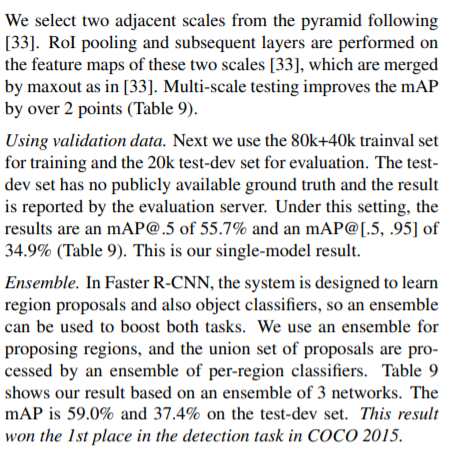
Using validation data. 다음으로 우리는 학습에 80k+40k trainval set 와 평가에 20k test-dev set를 사용한다. testdev set에서 공개적으로 사용할 수 있는 ground truth가 없으며 결과는 evaluation server에 의해 보고된다. 이 설정 하에서 결과는 mAP@.5 of 55.7% and an mAP@[.5, .95] of 34.9% (Table 9)이다. 이것은 우리의 single-model result이다.
Ensemble. Faster R-CNN에서 시스템은 region proposals과 object classifiers를 학습하도록 설계되어 있으므로 ensemble 을 사용하여 두 작업을 모두 향상시킬 수 있다. 우리는 regions을 제안하기 위해 앙상블을 사용하고 , 제안의 union set는 per-region classifiers 에 의해 처리된다. Table 9는 3개의 networks의 ensemble을 기반으로 한 우리의 결과를 보여준다. mAP 는 test-dev set에서 59.0% and 37.4%이다. 이 결과는 2015년 COCO detection task에서 1위를 차지했다.
PASCAL VOC
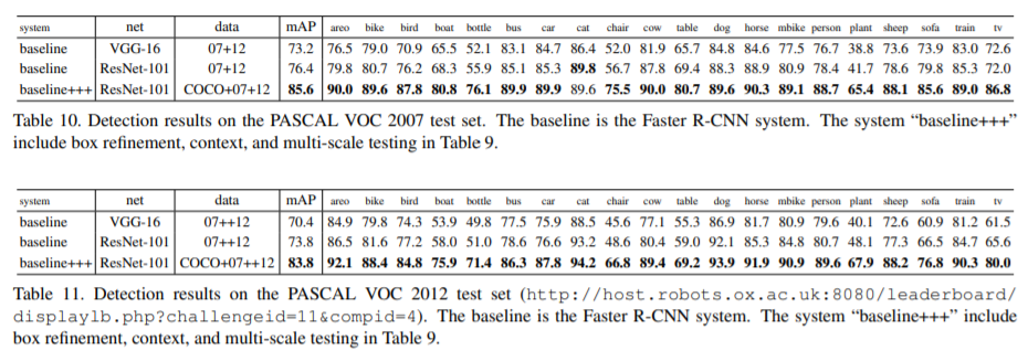
위의 모델을 기반으로 PASCAL VOC dataset를 다시 살펴본다. COCO dataset의 single model(55.7% mAP@.5 in Table 9) 를 사용하여 PASCAL VOC sets에서 이 모델을 fine-tune한다. box refinement, context, and multi-scale testing의 개선 사항도 채택되었다. 이를 통해 PASCAL VOC 2007 (Table 10) 85.6%를 달성하고 and PASCAL VOC 2012 (Table 11)에서 83.8% 를 달성했다. ASCAL VOC 2012에서의 결과는 이전의state-of-the-art result [6] 보다 더 높다.
ImageNet Detection
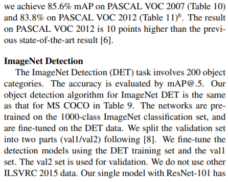
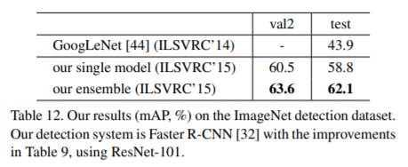
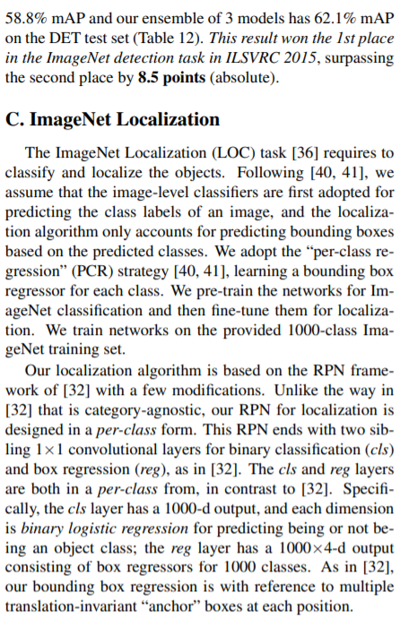
ImageNet Detection (DET) 작업은 200개의 object categories를 포함한다. 정확도는 mAP@.5로 평가된다. ImageNet DET 에 대한 우리의 object detection algorithm은 Table 9의 MS COCO와 동일하다. 이 networks 들은 1000-class ImageNet classification set에서 pretrained 되며 DET data에서 fine-tuned 된다. validation set 를 [8]에 이어 두 부분 (val1/val2)으로 분할했다. DET training set와 val1 set를 사용하여 detection models 을 fine-tune한다. val2 set 가 검증에 사용된다. ILSVRC 2015 data에서 사용하지 않는다. ResNet-101을 사용하는 single model 은 58.8%의 mAP를 가지며 3 models의 ensemble은 DET test set (Table 12)에서 2.1%의 mAP를 가진다(Table 12). 이 결과는 ILSVRC 2015에서 ImageNet detection task 1위를 차지해 2위를 8.5 points (absolute) 앞섰다.
C. ImageNet Localization
ImageNet Localization (LOC) task [36] 에서는 objects를 classify and localize를 요구한다. [40, 41]에 이어 , 우리는 image-level classifiers가 image의 class label을 예측하기 이해 먼저 채택되고 , localization algorithm 은 예측된 class를 기반으로 bounding boxes 예측만 설명한다고 가정한다. 우리는 각 class에 대한 bounding box regressor 를 학습하는 “per-class regression” (PCR) strategy [40, 41]을 채택한다. 우리는 ImageNet classification 를 위해 network를 pre-train 한 다음 localization을 위해 fine-tune한다. 제공된 1000-class ImageNet training set에서 network를 학습한다. 우리의 localization algorithm은 몇 가지 수정을 거친 [32] 의 RPN(Region proposal network) framework 를 기반으로 한다. category-agnostic [32]의 방식과 달리, localization 에 대한 RPN 은 per-class form으로 설계되었다. 이 RPN 은 [32]에서와 같이 binary classification (cls) and box regression (reg)를 two sibling 1×1 convolutional layers로 끝난다. [32]와 대조적으로 , cls와 reg layers은 둘 다 per-class에 있다. 특히 cls layer는 1000-d output를 가지며 , 각 차원은 object class 유무를 예측하기 위한 binary logistic regression이다 ; [32]에서와 같이 bounding box regression는 각 위치에 있는 multiple translation-invariant “anchor” boxes 를 참조한다.
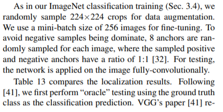
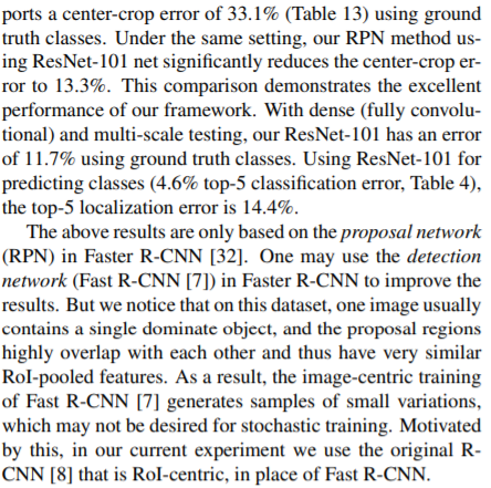
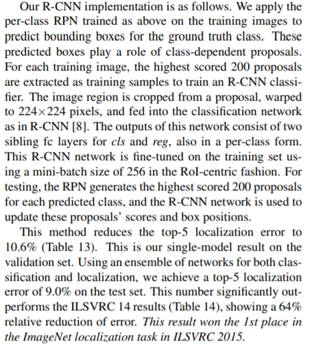
ImageNet classification training (Sec. 3.4)에서 처럼 data augmentation를 위해 224×224 crops 을 무작위로 샘플링한다. fine-tuning을 위해 256 images 의 mini-batch size를 사용한다. negative samples이 지배되는 것을 방지하기 위해 각 이미지에 대해 8개의 anchors 를 샘플링하며 , 여기서 샘플링된 positive and negative anchors의 비율은 1:1 [32]이다. 테스트를 위해 network는 image fully-convolutionally 적용된다. Table 13은 localization results를 비교한다. [41]에 이어 먼저 classification prediction으로 ground truth class를 사용하여 “oracle” testing를 수행한다. VGG’s paper [41]은 ground truth classes를 사용하여 33.1% (Table 13) 의 center-crop error를 보고한다. 동일한 설정에서 , ResNet-101 net을 사용하는 RPN method은 center-crop error를 13.3 %로 크게 줄인다. 이 비교는 우리 framework의 우수한 성능을 입증한다. dense (fully convolutional)및 multi-scale testing에서 ResNet-101은 ground truth classes를 사용하여 11.7%의 error를 가진다. classes 예측에 ResNet-101사용할 경우 (4.6% top-5 classification error, Table 4) , top-5 localization error is 14.4%이다.
위의 결과는 Faster R-CNN [32]의 roposal network (RPN)에만 기반한다. 결과를 개선하기 위해 Faster R-CNN의 detection network (Fast R-CNN [7])를 사용할 수 있다. 그러나 이 dataset에서는 일반적으로 하나의 이미지가 하나의 dominate object를 포함하고 proposal regions 이 서러 매우 겹쳐서 매우 유사한 ROI 풀 기능을 가지고 있다는 것을 알 수 있다. 결과적으로 , Fast R-CNN [7]의 image-centric training은 stochastic training에는 바람직하지 않을 수 있는 작은 변화의 샘플을 생성하다. 이에 자극을 받아 current experiment에서는 Fast R-CNN 대신 RoI-centric의 original RCNN [8]을 사용한다.
우리의 R-CNN 구현은 다음과 같다. 우리는 training images 에 위에서 학습된 per-class RPN을 적용하여 ground truth class에 대한 경계 상자를 예측한다. 이러한 predicted boxes는 class-dependent proposals의 역할을 한다. 각 training image에 대해 가장 높은 점수를 받은 200 proposals이 R-CNN classifier를 학습하기 이한 학습 샘플로 추출된다. image region은 proposal에서 cropped내어 224×224 pixels로 뒤틀린 다음 R-CNN [8]에서와 같이 classification network에 공급된다. 이 network의 출력은 cls와 reg에 대한 두개의 sibling fc layers으로 구성되며 , per-class form로도 구성된다. 이 R-CNN network 는 RoI-centric fashion의 방식으로 256개의 mini batch size를 사용하여 training set에서 fine-tuned 된다. testing를 위해 RPN은 각 예측 클래스에 대해 가장 높은 점수를 200 proposals 을 생성하고 , R-CNN network를 사용하여 이러한 proposals’ scores and box positions을 업데이터한다.
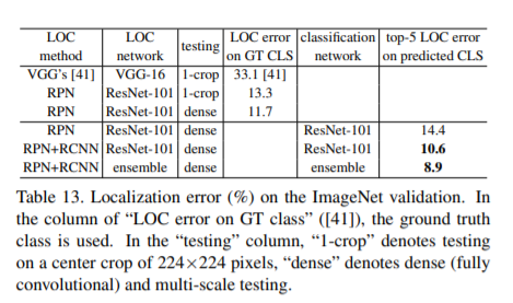
이 방법은 top-5 localization error를 10.6% (Table 13) 줄였다. 이것은 validation set에 대한 우리의 single-model result 이다. lassification and localization에 network ensemble 을 사용하여 test set에서 top-5 localization error of 9.0%에 이른다. 이 수치는 ILSVRC 14 results (Table 14)를 크게 능가하며, 상대적인 error 감소를 보여준다. 이 결과는 ILSVRC 2015에서 ImageNet localization task에서 1위를 차지했다.
Deep residual networks 는 매우 deep architectures 으로 등장하여 compelling accuracy and nice convergence behaviors 의 특성을 가지는 것을 알 수 있다.여기에서 우리는 the propagation formulations behind the residual building blocks 분석하며 , which suggest that the forward and backward signals can be directly propagated from one block to any other block, when using identity mappings as the skip connections and after-addition activation.
일련의 ablation experiments은 these identity mappings에서 중요한 역할을 하는 것을 검증한다. 이것으로 하여 우리는
a new residual unit를 제안하였으며 , 이 것으로 하여 우리는 학습을 쉽고 일반화를 높일 수 있게 하였습니다.
improved 결과 :
a 1001-layer ResNet on CIFAR-10 (4.62% error) and CIFAR-100
Deep residual networks (ResNets) 은 여러개 “Residual Units” 로 쌓여있는 형태이다.
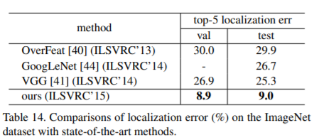
Each unit 의 보통 form
F is a residual function.
h(xl) = xl is an identity mapping and f is a ReLU [2] function.
identity mapping :항등 함수(恒等函數,영어:identity function) 또는항등 사상(恒等寫像,영어:identity map),항등 변환(恒等變換,영어:identity transformation)은정의역과공역이 같고, 모든 원소를 자기 자신으로 대응시키는함수이다.
ResNets that are over 100-layer 을 사용하여 우리는 several challenging recognition tasks on ImageNet [3] and MS COCO [4] competitions에서 높은 정확도가 나왔는지 알 수 있다. ResNets의 핵심 사상은 to learn the additive residual function F with respect to h(xl), with a key choice of using an identity mapping h(xl) = xl .이것은 identity skip connection (“shortcut”) 첨가하여 실현하였다.
In this paper, we analyze deep residual networks by focusing on creating a “direct” path for propagating information — not only within a residual unit, but through the entire network. Our derivations reveal that if both h(xl) and f(yl) are identity mappings, the signal could be directly propagated from one unit to any other units, in both forward and backward passes. 우리의 실험 경험적으로 볼 때 , 이 architecture 가 두가지 상태에 가까울 때 , 학습이 좀 더 간단해졌다.
To understand the role of skip connections, we analyze and compare various types of h(xl).
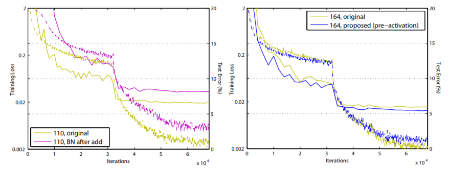
Figure 1. Left: (a) original Residual Unit in [1]; (b) proposed Residual Unit. The grey arrows indicate the easiest paths for the information to propagate, corresponding to the additive term “xl” in Eqn.(4) (forward propagation) and the additive term “1” in Eqn.(5) (backward propagation). Right: training curves on CIFAR-10 of 1001-layer ResNets. Solid lines denote test error (y-axis on the right), and dashed lines denote training loss (y-axis on the left). The proposed unit makes ResNet-1001 easier to train.
우리는 skip connections 의 역할을 이해하기 위하여 , 우리는 여러가지 타입의 h(xl) 비교하면서 분석하였다. 우리는 identity mapping h(xl) = xl 선택하여 사용해서 우리가 연구한 모든 유형중에서 , 빠른 error reduction과 최저의 training loss among all variants , whereas skip connections of scaling, gating [5,6,7], and 1×1 convolutions all lead to higher training loss and error. 이들 실험 제안으로 , that keeping a “clean” information path (indicated by the grey arrows in Fig. 1, 2, and 4) is helpful for easing optimization.
an identity mapping f(yl) = yl 구조를 위하여 , 우리는 the activation functions (ReLU and BN [8]) as “pre-activation” ” of the weight layers, conventional wisdom of “post-activation”와 대조하다. 이 점을 통하여 우리는 새로운 residual unit 이 설계되여서 , shown in (Fig. 1(b)). 이 unit을 기존으로 , 우리는 we present competitive results on CIFAR-10/100 with a 1001-layer ResNet, 이것은 많이 쉽게 학습과 일반적으로 original ResNet 보다 학습하기 좋다. ImageNet using a 200-layer ResNet에 대하여 overfit방식이 나타나서 , 우리는 더 나은 것을 표현하기 위하여 개조한 인터넷 결과를 사용하였다. 결과로 인하여 , 심도있게 학습이 성공의 중요 포인터이고 , 모델의 deep learning 은 아직도 더 큰 dimension of network depth있다.
2 Analysis of Deep Residual Networks
ResNets는 같은 connecting shape 를 통하여 bloks을 stack building으로 모듈화 아키텍츠를 만든다. 여기에서는 우리는 이 blocks를 "Residual Units"이라고 한다.
original Residual Unit in [1] performs the following computation:
xl : the input feature to the l-th Residual Unit.
Wl = {Wl,k|1≤k≤K} : a set of weights (and biases) associated with the l-th Residual Unit
K : the number of layers in a Residual Unit (K is 2 or 3 in [1])
F denotes the residual function, e.g., a stack of two 3×3 convolutional layers in [1]
function f: the operation after element-wise addition
f is ReLU
function h : set as an identity mapping: h(xl) = xl
만약 f 는 also an identity mapping: xl+1 ≡ yl , we can put Eqn.(2) into Eqn.(1) and obtain:
Recursively (xl+2 = xl+1 + F(xl+1, Wl+1) = xl + F(xl , Wl) + F(xl+1, Wl+1), etc.) we will have:
for any deeper unit L and any shallower unit l.Eqn.(4)는 exhibits some nice properties. (i) The feature xL of any deeper unit L can be represented as the feature xl of any shallower unit l plus a residual function in a form of
, 이것은 any units L and l 사이에서는 모두 residual fashion특성 을 가지고 있다 . (ii)
Eqn. : 영어에서 변역됨 -Unix문서 레이아웃 도구의 troff제품군의 일부인 eqn 은 인쇄 방정식을 형식화하는 전 처리기입니다.
Eqn.(4) also leads to nice backward propagation properties. loss function을 E으로 표시하고 , from the chain rule of backpropagation [9] we have:
두가지로 분해 할 수 있다.
그중에서 앞에것은 직접 신호를 전하고 아무른 weight layers와 관계가 없다. 다른 한가지는 propagates through the weight layers . 앞에것은 신호가 직접 다른 shallower unit l의 전달을 보장해준다.
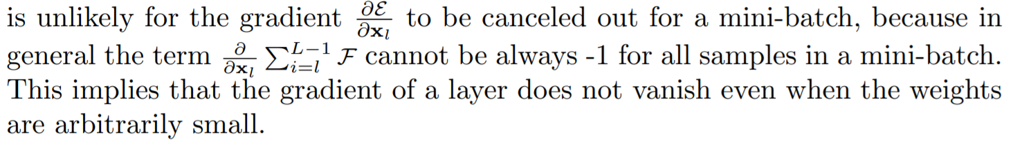
이것은 weight가 아무리 작어도 , gradient는 소실하지 않는 현상이 생긴다.
Discussions
Eqn.(4) and Eqn.(5)은 both forward and backward 단계에서 , 신호는 직접 이 unit에서 임의의 다른 unit으로 직접 전달 할 수 있다.
The foundation of Eqn.(4) is two identity mappings:
(i) the identity skip connection h(xl) = xl
(ii) the condition that f is an identity mapping
이들 directly propagated information flows은 Fig. 1, 2, and 4에서 grey arrows로 표시한 것으로 한다. these grey arrows cover no operations (expect addition) and thus are “clean” 일 경우 , 위의 두가지 조건은 성립된다. 아래의 두 부분에서는 우리는 두가지 조건의 작용에 대하여 갈라서 결과를 연구한다.
3 On the Importance of Identity Skip Connections
간단한 수정을 설계한다. h(xl) = λlxl 으로 to break the identity shortcut:
λl : a modulating scalar (for simplicity we still assume f is identity).
여기서 재귀적으로 지원해서 푼다면 Eqn. (4)와 비슷한 것을 얻는다 :
그중 the scalars into the residual functions를 합친다. 이것은 Eq.5 와 비슷하다. 우리는 backpropagation의 전파 과정은 위의 겉과 같다.
Eq.5와 같지 않게 , Eq.8중에서 first additive term 은 요소에 따라 변조한다.
극단적인 deep network중에서 (L은 매우 크다)
만약 λi > 1 for all i : 요소들은 exponentially 클 수 있다.
만약 λi < 1 for all i : 요소들은 exponentially 작아지거나 소실 할 수 있다. which blocks the backpropagated signal from the shortcut and forces it to flow through the weight layers. 우리는 실험을 통해 optimazation 의 우화를 어렵게 할 수 있다는 것을 증명하였다.
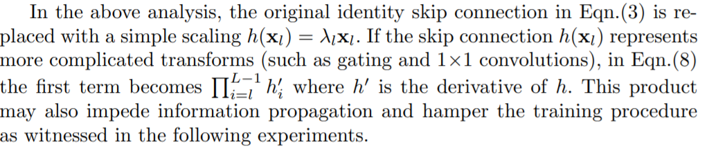
위의 분석중 , Eqn.(3)중의 original identity skip connection 은 with a simple scaling h(xl) = λlxl로 대체할 수 있다.
만약 skip connection h(xl)은 더욱 복잡하게 변형한다는 것을 대표한다면 s (such as gating and 1×1 convolutions),
in Eqn.(8) the first term 은 방정식으로 표현한다. 이런 성적으로는 똑 같이 information propagation 방해하고 and hamper the training procedure 아래의 실험에서 우리는 익서을 증명할 수 있다.
Figure 2. Various types of shortcut connections used in Table 1. The grey arrows indicate the easiest paths for the information to propagate. The shortcut connections in (b-f) are impeded by different components. For simplifying illustrations we do not display the BN layers, which are adopted right after the weight layers for all units here.
Figure 2 Table 1에서의 여러가지 타입의 shortcut 을 연결한다. greay arrow에서는 정보전파의 최단거리를 표시한다 . (b-f)중에서 sortcut연결은 다른 같지 않은 성분으로 방행하였다. 간단하게 할려고, 우리는 BN layers를 그리지 않고 이것은 weight layers의 뒤에 연결해야 한다.
3.1 Experiments on Skip Connections
우리는 110-layer ResNet 에서 CIFAR-10을 사용하였다.
extremely deep ResNet-110 :
54 two-layer Residual Units (consisting of 3×3 convolutional layers)
challenging for optimization
우리의 실험 자세한 정보는 ((see appendix ) are the same as [1]. random variations의 영향을 피하기 위하여 , 여기에서 우리는 5 runs for each architecture on CIFAR 중 median accuracy을 결과로 하였다.
위의 분석중 f는 identity mappeng으로 하였지만 , 여기에서 실험할 경우 f = ReLU으로 모두 하였다 , 다음 부분부터 우리는 identity f 로 분석을 진행한다. 우리의 baseline ResNet-110 는 6.61% error on the test set 가 있다. 다른 variants와 비교하는것은 s (Fig. 2 and Table 1) 에서 요약한것과 같다:
Table 1. Classification error on the CIFAR-10 test set using ResNet-110 [1], with different types of shortcut connections applied to all Residual Units. We report “fail” when the test error is higher than 20%.
Constant scaling.
모든 shortcuts의 연결중 λ = 0.5 , 우리는 더욱이 F 를 두가지 scaling 으로 고려한다.:
(i) F is not scaled; => 이 caset는 does not converge well
(ii) F is scaled by a constant scalar of 1−λ = 0.5, which is similar to the highway gating [6,7] but with frozen gates.=> is able to converge, but the test error (Table 1, 12.35%) is substantially higher than the original ResNet-110.
Fig 3(a) shows that the training error is higher than that of the original ResNet-110, suggesting that the optimization has difficulties when the shortcut signal is scaled down.
Exclusive gating.
Following the Highway Networks [6,7] that adopt a gating mechanism [5], 우리는 gating function을 고려한다. weight, biases, sigmoid함수로 변환하면서 한다. convolutional network g(x)중 1×1 convolutional layer을 통과하여 실현한다. gating 함수는 element-wise 곱하여 신호를 조절한다.
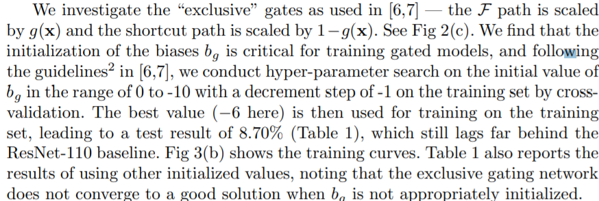
우리는 investigate the “exclusive” gates as used in [6,7] — — the F path is scaled by g(x) and the shortcut path is scaled by 1−g(x). See Fig 2(c). 우리는 초기화 biase가 중요한 학습 gated의 모듈인것과 가이드라인에 따라 하는 것이 중요하다는 것을 발견하였다. 우리는 bias를 0부터 10 까지를 초기화 범위로 하고 , 하나씩 줄이고 그다음 cross-validation방법을 통해 hyper-parameter을 찾으면서 실행하였다. 그리고 최적 의 갓ㅂ으로 훈련하여 , leading to a test result of 8.70% (Table 1), 그래도 original ResNet-110보다 휠씬 뒤떨어져있다. Fig 3(b)은 훈련과정을 표시한다. Table 1도 다른 초기화 값을 이용하여 실험환 결과를 보여주고 , bg의 초기화 값이 합법적이지 않을 경우 exclusive gating does not converge to a good solution하는것을발견하였다.
exclusive gating mechanism은 two-fold 영향을 받는다.
1 − g(x) 가 1에 가까울때 , the gated shortcut connections are closer to identity which helps information propagation; =>신호 전달에 도움이 된다.
g(x) approaches 0 and suppresses the function F. To isolate the effects of the gating functions on the shortcut path alone, we investigate a non-exclusive gating mechanism in the next.
Shortcut-only gating. function F is not scaled; only the shortcut path is gated by 1−g(x). See Fig 2(d). initialized value of bg는 이 case에도 여전히 중요하다.
When the initialized bg is 0 (so initially the expectation of 1 − g(x) is 0.5), the network converges to a poor result of 12.86% (Table 1). This is also caused by higher training error (Fig 3(c)). 낮다.
Figure 3. Training curves on CIFAR-10 of various shortcuts. Solid lines denote test error (y-axis on the right), and dashed lines denote training loss (y-axis on the left).
When the initialized bg is very negatively biased (e.g., −6), 1−g(x)의 값이 1에 가깝고 and the shortcut connection is nearly an identity mapping.
1×1 convolutional shortcut. Next we experiment with 1×1 convolutional shortcut connections that replace the identity. 이 선택적 방안은 34-layer ResNet(16 Residual Units)에 사용(option C )하였고 좋은 결과를 가질 뿐만 아니라 ,suggesting that 1×1 shortcut connections could be useful. 하지만 우리는 this is not the case when there are many Residual Units인 것을 발견하였다. 1×1 convolutional shortcuts을 사용할 경우 110-layer ResNet 은 좋지 않은 결과가 나왔다(12.22%, Table 1 ). Again, the training error becomes higher (Fig 3(d)). stacking so many Residual Units (54 for ResNet-110)일 경우 , the shortest path일지라도 신호 propagation을 방해한다. 우리는 on ImageNet with ResNet-101 when using 1×1 convolutional shortcuts 일 경우 비슷한 결과를 나타났다.
Dropout shortcut. 마지막으로 우리는 dropout [11] (at a ratio of 0.5) which we adopt on the output of the identity shortcut (Fig. 2(f))으로 실험한다 . The network fails to converge to a good solution. Dropout 통계적으로 imposes a scale of λ with an expectation of 0.5 on the shortcut, and similar to constant scaling by 0.5, 똑같이 signal propagation을 방해한다.
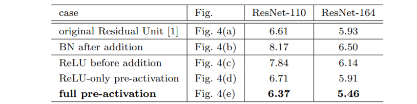
Table 2. Classification error (%) on the CIFAR-10 test set using different activation functionsFigure 4. Various usages of activation in Table 2. All these units consist of the same components — only the orders are different.
3.2 Discussions
Fig. 2의 회식 arrow중 표시한듯이 , shortcut connections는 정보 전파 중 제일 직접적인 경로이다.
Multiplicative manipulations (scaling, gating, 1×1 convolutions, and dropout) on the shortcuts can hamper information propagation 과 optimization 문제가 생긴다.
주목해야 할 점은 the gating and 1×1 convolutional shortcuts은 더 많은 파라미터를 설명하였고 ,
identity shortcuts보다 더 강한 표현 능력이 있어햐 한다. 사실은 shortcut-only gating 와 1×1 convolution over the solution space of identity shortcuts (i.e., they could be optimized as identity shortcuts). 하지만 , their training error 는 identity shortcuts보다 훨씬 높아서 , degradation of these models 을 나타나며 원인은 optimazation issues, 표현 능력의 문제가 아니다 .
4 On the Usage of Activation Functions
위의 실험내용에서 우리는 Eqn.(5) and Eqn.(8)의 내용에 대해 분석하고 , 두가지 공식은 전부 both being derived under the assumption that the after-addition activation f is the identity mapping. 하지만 위의 실험에서 f is ReLU as designed in [1], so Eqn.(5) and (8) are approximate in the above experiments. 다음에 우리는 f 의 영향에 대해 연구한다.
우리는 re-arranging the activation functions (ReLU and/or BN)을 통하여 f를 identity mapping 으로 하고 싶다. The original Residual Unit 의 모양은 Fig.4(a) 중 처럼 BN은 매 weight layer중 사용하고 그다음 ReLU, 그리고 마지막에 element-wise를 추가하고 마지막에 ReLU(f=f=ReLU)추가한다. Fig.4(b-e)는 우리가 연구한 다른 모양을 해설하였다.
4.1 Experiments on Activation
우리는 ResNet-110 and a 164-layer Bottleneck [1] architecture (denoted as ResNet-164)으로 실험하였다 . A bottleneck Residual Unit 는 1×1 layer for reducing dimension으로 포함되였고 , , a 3×3 layer, and a 1×1 layer for restoring dimension(차원 복원). As designed in [1], 계산 복잡도는 two-3×3 Residual Unit과 비슷하다. 더 자세하게는 in the appendix에 있다. The baseline ResNet164 has a competitive result of 5.93% on CIFAR-10 (Table 2).
BN after addition. Before turning f into an identity mapping , we go the opposite way by adopting BN after addition (Fig. 4(b)). 이 케이스에서는 f는 BN과 ReLU가 포함되였다. 이 결과는 baseline의 결과보다 훨 낮다(Table2). 원래의 original 설계와 다르게, now BN layer 는 지나가는 경로의 the shortcut 신호를 변하게 하고 정보 propagation을 방해하고 , 이것은 훈련 처음 부터 reducing training loss의 힘드는 것을 보인다(Fig.6 left).
ReLU before addition. f into an identity mapping 의 소박한 선택은 ReLU를 Addition 전으로 이동한다(Fig. 4(c)).하지만 , the transform F의 output이 non-negative으로 하고 , while intuitively a “residual” function should take values in (−∞, +∞). 이 결과를 얻는 이유는 he forward propagated signal is monotonically increasing . 이것은 표현 능력에 영향을 주고 , 결과를 baseline보다 더욱 나쁘게 한다(7.84%, Table 2). 우리는 잔차함수가 (−∞, +∞)의 값 사이에 있기를 희망한다. 이 조건은 n is satisfied by other Residual Units including the following ones.
원래의 설계중 , 활성화 함수는 두가지 길에서 다음희 Residual Unit에서 영향을 준다.
그다음 우리는 asymmetric 방식을 연구
notation에 재명명을 통하여 우리는 위의 공식 형식을 얻을 수 있다.
우리는 쉽게 Eqn.(9) 과 Eqn.(4) 비슷하다는 것을 알 수 있어서 , 그래서 우리는 a backward formulation similar to Eqn.(5)을 얻을 수 있다. For this new Residual Unit as in Eqn.(9), he new after-addition activation는 an identity mapping을 으로 되였다. 이 설계의 의미는
Figure 5. Using asymmetric after-addition activation is equivalent to constructing a pre-activation Residual Unit.Table 3. Classification error (%) on the CIFAR-10/100 test set using the original Residual Units and our pre-activation Residual Units.
post-activation/pre-activation 사이의 차이는 the presence of the element-wise addition가 원인이다. For a plain network that has N layers, there are N − 1 activations (BN/ReLU), and it does not matter whether we think of them as post- or pre-activations. 하지만 우리가 추가한 branch layer으로 말하면 , the position of activation matters.
우리는 아래의 두가지 설계를 사용하여 실험을 진행하였다:
(i) ReLU-only pre-activation (Fig. 4(d)), and (ii) full pre-activation (Fig. 4(e)) where BN and ReLU are both adopted before weight layers. Table 2는 the ReLU-only pre-activation performs와 the baseline on ResNet-110/164 비슷하다는 것을 표시하였다. 이 ReLU layer는 BN layer과 연결하여 사용하지 않아서 , 그래서 may not enjoy the benefits of BN [8].
Figure 6. Training curves on CIFAR-10. Left: BN after addition (Fig. 4(b)) using ResNet-110. Right: pre-activation unit (Fig. 4(e)) on ResNet-164. Solid lines denote test error, and dashed lines denote training loss.
하지만 놀랍게도 , 우리가 BN과 ReLU가 pre-activation을 다 사용할 경우, 그 결과는 improved by healthy margins (Table 2 and Table 3). In Table 3 we report results using various architectures: (i) ResNet-110, (ii) ResNet-164, (iii) a 110-layer ResNet architecture in which each shortcut skips only 1 layer (i.e.,a Residual Unit has only 1 layer), denoted as “ResNet-110(1layer)”, and (iv) a 1001-layer bottleneck architecture that has 333 Residual Units (111 on each feature map size), denoted as “ResNet-1001”. We also experiment on CIFAR100.Table 3 에서 우리의 “pre-activation” models 은 일관되게 baseline counterparts의 보다 좋다. 분석 과정은 아래와 같다.
4.2 Analysis
우리는 pre-activation의 영향은 두가지를 가지고 있는 것을 발견하였다.
첫째 , f는 identity mapping 이기 때문에 the optimization is further eased (comparing with the baseline ResNet)
둘째 , using BN as pre-activation improves regularization of the models.
Ease of optimization. 우리는 1001-layer ResNet 을 훈련한 경우 매우 선명하게 영향을 가지고 있다. Fig. 1 shows the curves. original design in [1]을 사용하여 , training error는 처음에 훈련할 경우 매우 천천히 줄어든다. for f=f=ReLU, 만약 negative일 경우 신호는 방해되고 , 그리고 여러가지 Residual Units이 있을 경우 , this effect becomes prominent and Eqn.(3) (so Eqn.(5)) is not a good approximation. 다른 한편으로는 f가 identity mapping 일 경우 , 신호는 can be propagated directly between any two units. 우리의 1001-layer network는 training loss를 낮추는데 매우 빠르다(Fig.1).
It also achieves the lowest loss among all models we investigated, suggesting the success of optimization.
We also find that the impact of f = ReLU is not severe when the ResNet has fewer layers (e.g., 164 in Fig. 6(right)). beginning of training 에서 training curve 는 조금만 영향을 가지는 것 같지만 , 하지만 goes into a healthy status soon. 모니터링을 통해 우리는 관찰되였는데, 원인은 일정한 훈련을 통해, the weights are adjusted into a status such that yl in Eqn.(1) is more frequently above zero and f does not truncate it (xl is always non-negative due to the previous ReLU, so yl is below zero only when the magnitude of F is very negative).The truncation, however, is more frequent when there are 1000 layers.
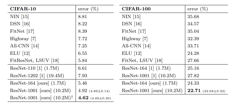
Table 4. Comparisons with state-of-the-art methods on CIFAR-10 and CIFAR-100 using “moderate data augmentation” (flip/translation), except for ELU [12] with no augmentation. Better results of [13,14] have been reported using stronger data augmentation and ensembling. For the ResNets we also report the number of parameters. Our results are the median of 5 runs with mean±std in the brackets. All ResNets results are obtained with a mini-batch size of 128 except † with a mini-batch size of 64 (code available at https://github.com/KaimingHe/resnet-1k-layers).
Reducing overfitting. Another impact of using the proposed pre-activation unit is on regularization, as shown in Fig. 6 (right). The pre-activation version reaches slightly higher training loss at convergence, but produces lower test error. 이 현상은 on ResNet-110, ResNet-110(1-layer), and ResNet-164 on both CIFAR-10 and 100에서 관찰 할 수 있다. 이것은 아마도 BN’s regularization effect [8]이 원인이다. In the original Residual Unit (Fig. 4(a)), BN normalizes 는 신호이지만 , this is soon added to the shortcut and thus the merged signal is not normalized. 이 빙정규화 신호는 또 다음의 weight layers의 입력에 의해 사용된다. . On the contrary, in our pre-activation version, all weight layers 의 입력은 normalized로 되여있다.
5 Results
Comparisons on CIFAR-10/100.. Table 4 에서 CIFAR-10/100를 최근의 잴 좋은 방법으로 비교하여 , 우리의 모델 은 매우 경쟁성이 있는 결과를 얻었다. 우리는 these small datasets 에 대해서 , 우리는 특별하게 tailor the network width or filter sizes 할 필요 없고 , 정규화 기술을 사용(such as dropout)할 필요 없이 모델의 효과를 보장하였다. 우리는 단지 간단하고 효과있는 방식을 통하여 -------- going deeper. 이것들의 결과는 demonstrate the potential of pushing the limits of depth.
Table 5. Comparisons of single-crop error on the ILSVRC 2012 validation set. All ResNets are trained using the same hyper-parameters and implementations as [1]). Our Residual Units are the full pre-activation version (Fig. 4(e)). † : code/model available at https://github.com/facebook/fb.resnet.torch/tree/master/pretrained, using scale and aspect ratio augmentation in [20].
Comparisons on ImageNet. 다음에 우리는 1000- class ImageNet dataset [3]에서 실험결과를 보여준다. We have done preliminary experiments using the skip connections studied in Fig. 2 & 3 on ImageNet with ResNet-101 [1], and observed similar optimization difficulties. The training error of these non-identity shortcut networks is obviously higher than the original ResNet at the first learning rate(similar to Fig. 3), 자원이 한정되여있어서 우리는 절반을 학습하기로 결정하였다. 하지만 우리는 “BN after addition” version (Fig. 4(b)) of ResNet-101 on ImageNet and observed higher training loss and validation error을 완성하였다. This model’s single-crop (224×224) validation error is 24.6%/7.5%, vs. the original ResNet101’s 23.6%/7.1%. 이것은 Fig. 6 (left)에서 CIFAR의 결과와 같다.
Table 5는 the results of ResNet-152 [1] and ResNet-2003 을 표시하며 , 전부 처음 부터 학습하였다. We notice that the original ResNet paper [1] trained the models using scale jittering with shorter side s ∈ [256, 480], and so the test of a 224×224 crop on s = 256 (as did in [1]) is negatively biased. Instead, we test a single 320×320 crop from s = 320, for all original and our ResNets. Even though the ResNets are trained on smaller crops, they can be easily tested on larger crops because the ResNets are fully convolutional by design. This size is also close to 299×299 used by Inception v3 [19], allowing a 공평한 비교이다.
The original ResNet-152 [1] has top-1 error of 21.3% on a 320×320 crop, and our pre-activation counterpart has 21.1%. The gain is not big on ResNet-152 because this model has not shown severe generalization difficulties.하지만 original ResNet-200 의 error rate of 21.8%이고 , baseline ResNet-152보다 높다. . But we find that the original ResNet-200 has lower training error than ResNet-152, suggesting that it suffers from overfitting.
우리의 pre-activation ResNet-200 의 error rate는 20.7%, which is 1.1% lower than the baseline ResNet-200 and also lower than the two versions of ResNet-152. When using the scale and aspect ratio augmentation of [20,19], our ResNet-200 has a result better than Inception v3 [19] (Table 5). Concurrent with our work, an Inception-ResNet-v2 model [21] achieves a single-crop result of 19.9%/4.9%. We expect our observations and the proposed Residual Unit will help this type and generally other types of ResNets.
Computational Cost. 우리의 모델의 계산복잡도와 depth는 linear관계를 가진다(so a 1001-layer net is ∼10× complex of a 100-layer net). On CIFAR, ResNet-1001 takes about 27 hours to train on 2 GPUs; on ImageNet, ResNet200 takes about 3 weeks to train on 8 GPUs (on par with VGG nets [22]).
6 Conclusions
이 paper에서는 the propagation formulations behind the connection mechanisms of deep residual networks을 여구하였다. Our derivations imply that identity shortcut connections and identity after-addition activation are essential for making information propagation smooth. 제거 실험(Ablation experiments) demonstrate phenomena that are consistent with our derivations. 우리는 동시에 1000-layer deep networks을 제안하여 that can be easily trained and achieve improved accuracy.
Appendix: Implementation Details
The implementation details and hyperparameters are the same as those in [1]. On CIFAR we use only the translation and flipping augmentation in [1] for training. learning rate는 0.1부터 시작하여, and is divided by 10 at 32k and 48k iterations. Following [1], for all CIFAR experiments we warm up the training by using a smaller learning rate of 0.01 at the beginning 400 iterations and go back to 0.1 after that, although we remark that this is not necessary for our proposed Residual Unit. The mini-batch size is 128 on 2 GPUs (64 each), the weight decay is 0.0001, the momentum is 0.9, and the weights are initialized as in [23].
On ImageNet, we train the models using the same data augmentation as in [1]. The learning rate starts from 0.1 (no warming up), and is divided by 10 at 30 and 60 epochs. The mini-batch size is 256 on 8 GPUs (32 each). The weight decay, momentum, and weight initialization are the same as above.
When using the pre-activation Residual Units (Fig. 4(d)(e) and Fig. 5), we pay special attention to the first and the last Residual Units of the entire network. For the first Residual Unit (that follows a stand-alone convolutional layer, conv1), we adopt the first activation right after conv1 and before splitting into two paths; for the last Residual Unit (followed by average pooling and a fullyconnected classifier), we adopt an extra activation right after its element-wise addition. These two special cases are the natural outcome when we obtain the pre-activation network via the modification procedure as shown in Fig. 5.
Very deep convolutional networks with hundreds of layers 는 competitive benchmarks에서 오류를 크게 감소 할 수 있습니다. Although the unmatched expressiveness of the many layers can be highly desirable at test time, training very deep networks comes with its own set of challenges. 하지만 여러 가지 문제점이 있다.
1). gradients can vanish,
2). the forward flow often diminishes
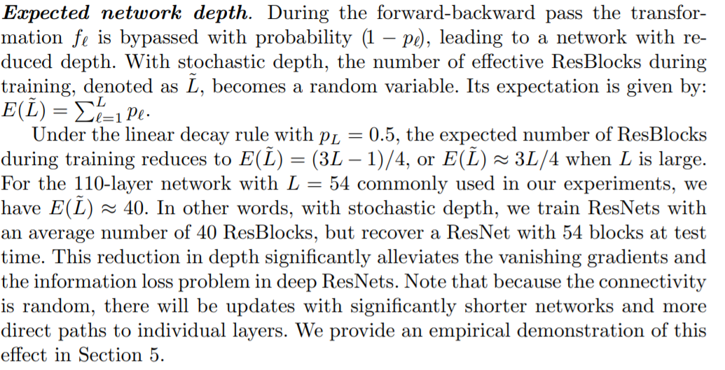
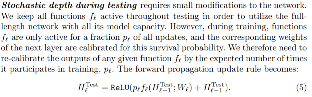
3). the trainning time can be painfully slow
이를 해결하기 위해 우리는 stochastic depth, a training procedure that enables the seemingly contradictory setup to train short networks and use deep networks at test time.
여기에서 우리는 먼저 very deep networks 시작하고 여러개의 mini-batch로 학습하며 , randomly drop a subset of layers and bypass them with the identify function. 이 간단한 접근으로 보완하여 최근의 resisual networks에 성공하였다. training time의 시간을 줄이고 대체로 거의 모든 data sets에서 테스트 오류를 크게 개선하여 평가에 사용합니다. With stochastic depth 우리는 the depth of residual networks의 층을 늘일 수 있고 even beyond 1200 layers and still yield meaningful improvements in test error (4.91% on CIFAR-10).
1 Introduction
Convolutional Neural Networks (CNNs)
computer vision [3, 4, 5, 6, 7, 8]
AlexNet had 5 convolutional layers [1]
VGG network and GoogLeNet in 2014 had 19 and 22 layers respectively [5, 7]
ResNet architecture featured 152 layers [8]
computer vision: 컴퓨터 비전(Computer Vision)은 기계의 시각에 해당하는 부분을 연구하는 컴퓨터 과학의 최신 연구 분야 중 하나이다.
Network depth is a major determinant of model expressiveness, both in theory [9, 10] and in practice [5, 7, 8]. However, very deep models also introduce new challenges: vanishing gradients in backward propagation, diminishing feature reuse in forward propagation, and long training time.
determinant :행렬식 : 선형대수학에서 , 행렬식은 정사각 행렬에 스칼라를 대응시키는 함수의 하나이다.
Vanishing Gradients is a well known nuisance in neural networks with many layers [11].As the gradient information is back-propagated, repeated multiplication or convolution with small weights renders the gradient information ineffectively small in earlier layers. Several approaches exist to reduce this effect in practice, for example through careful initialization [12], hidden layer supervision [13], or, recently, Batch Normalization [14].
Diminishing feature reuse during forward propagation (also known as loss in information flow [15]) refers to the analogous problem to vanishing gradients in the forward direction. gradient 훈련하기 힘들다 . making it hard for later layers to identify and learn “meaningful” gradient directions. Recently, several new architectures attempt to circumvent this problem through direct identity mappings between layers, which allow the network to pass on features unimpededly from earlier layers to later layers [8, 15].
Long training time is a serious concern as networks become very deep.gpu를 사용해도 시간이 오래 걸린다.
The researcher is faced with an inherent dilemma:
shorter networks have the advantage that information flows efficiently forward and backward, and can therefore be trained effectively and within a reasonable amount of time. However, they are not expressive enough to represent the complex concepts that are commonplace in computer vision applications. 효율성
Very deep networks have much greather model complexity, but are very difficult to train in practice and require a lot of time and patience. 시간이 오래 걸린다.
In this paper, we propose deep networks with stochastic depth, a novel training algorithm that is based on the seemingly contradictory insight that ideally we would like to have a deep network during testing but a short network during training. We resolve this conflict by creating deep Residual Network [8] architectures (with hundreds or even thousands of layers) with sufficient modeling capacity; however, during training we shorten the network significantly by randomly removing a substantial fraction of layers independently for each sample or mini-batch. The effect is a network with a small expected depth during training, but a large depth during testing. Although seemingly simple, this approach is surprisingly effective in practice.
stochastic depth substantially reduces training time and test error (resulting in multiple new records to the best of our knowledge at the time of initial submission to ECCV).The reduction in training time can be attributed to the shorter forward and backward propagation, so the training time no longer scales with the full depth, but the shorter expected depth of the network.
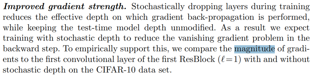
We attribute the reduction in test error to two factors: 1) shortening the (expected) depth during training reduces the chain of forward propagation steps and gradient computations, which strengthens the gradients especially in earlier layers during backward propagation; 2) networks trained with stochastic depth can be interpreted as an implicit ensemble of networks of different depths, mimicking the record breaking ensemble of depth varying ResNets trained by He et al. [8].
similar to Dropout [16], training with stochastic depth acts as a regularizer, even in the presence of Batch Normalization [14]. On experiments with CIFAR-10, we increase the depth of a ResNet beyond 1000 layers and still obtain significant improvements in test error.
2 Background
수많은 시도하에서 very deep networks 학습을 올릴 수 있었다.
Earlier works adopted greedy layer-wise training or better initialization schemes to alleviate the vanishing gradients and diminishing feature reuse problems [12, 17, 18].
주목할 만한 최근의 공헌으로는 very deep networks의 학습은 Batch Normalization을 이용한다.
Batch Normalization 는 which standardizes the mean and variance of hidden layers with respect to each mini-batch.
이 접근으로는 vanishing gradients problem을 줄일 수 있고 yields a strong regularizing effect.
최근에는 몇명의 저자들이 extra skip connections to improve the information flow during forward and backward propagation을 소계하였다. Highway Networks [15] allow earlier representations to flow unimpededly to later layers through parameterized skip connections known as “information highways”, which can cross several layers at once. The skip connection parameters, learned during training, control the amount of information allowed on these “highways”.
Residual networks (ResNets)[8] simplify Highway Networks by shortcutting (mostly) with identity functions.이것은 잴인 단순화하면서 잴 효과가 좋게 학습 효율을 높이며 enables more direct feature reuse. ResNets are motivated by the observation that neural networks tend to obtain higher training error as the depth increases to very large values.This is counterintuitive, as the network gains more parameters and therefore better function approximation capabilities.
The authors conjecture that the networks become worse at function approximation because the gradients and training signals vanish when they are propagated through many layers. => 여러 layers 을 통과할때
As a fix, they propose to add skip connections to the network.
Dropout. multiplies each hidden activation by an independent Bernoulli random variable.Intuitively, Dropout reduces the effect known as “coadaptation” of hidden nodes collaborating in groups instead of independently producing useful features; it also makes an analogy with training an ensemble of exponentially many small networks. Many follow up works have been empirically successful, such as DropConnect [20], Maxout [21] and DropIn [22].
with different depths, possibly achieving higher diversity among ensemble members than ensembling those with the same depth. Different from Dropout, we make the network shorter instead of thinner, and are motivated by a different problem. Anecdotally, Dropout loses effectiveness when used in combination with Batch Normalization [14, 23]. Our own experiments with various Dropout rates (on CIFAR-10) show that Dropout gives practically no improvement when used on 110-layer ResNets with Batch Normalization.
We view all of these previous approaches to be extremely valuable and consider our proposed training with stochastic depth complimentary to these efforts.
we show that training with stochastic depth is indeed very effective on ResNets with Batch Normalization.
3 Deep Networks with Stochastic Depth
stochastic depth 학습을 할 때는 간단한 직관을 기초로 한다. 학습을 할때 length of a neural network 효울성을 낮추기 위해서는 우리는 랜덤으로 skip layers entirely.
skip connections
connection pattern is randomly altered for each minibatch.
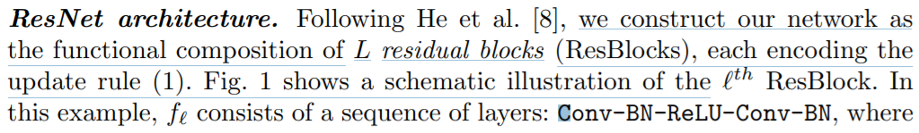
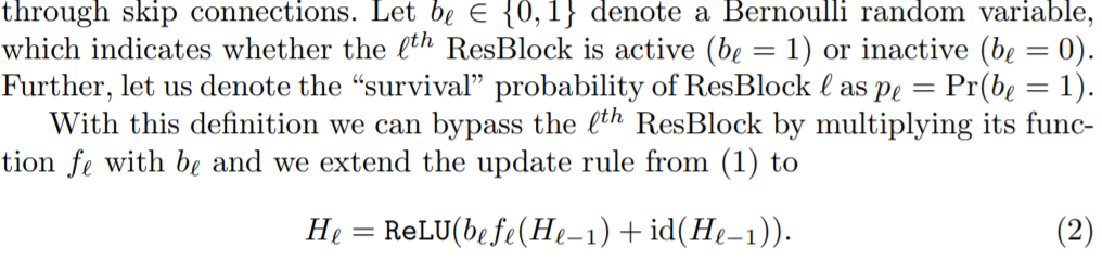
For each mini-batch we randomly select sets of layers and remove their corresponding transformation functions, only keeping the identity skip connection. Throughout, 우리는 He et al.가 묘사한 이 아키텍처를 사용한다. 왜냐하면 이 아케텍처는 원래 skip connections가 포함되여있고 it is straightforward to modify, and isolates the benefits of stochastic depth from that of the ResNet identity connections. Next we describe this network architecture and then explain the stochastic depth training procedure in detail.
Conv and BN stand for Convolution and Batch Normalization respectively. This construction scheme is adopted in all our experiments except ImageNet, for which we use the bottleneck block detailed in He et al. [8]. Typically, there are 64, 32, or 16 filters in the convolutional layers (see Section 4 for experimental details).
Conv-BN-ReLU-Conv-BN
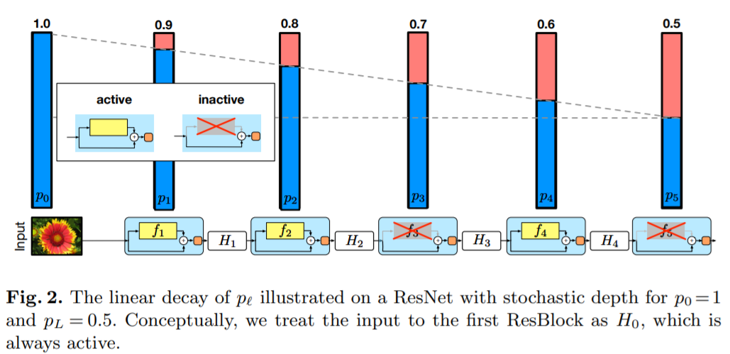
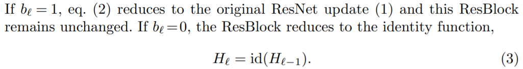
Stochastic depth aims to shrink the depth of a network during training, while keeping it unchanged during testing. We can achieve this goal by randomly dropping entire ResBlocks during training and bypassing their transformations
Bernoulli random variable :
베르누이 분포(Bernoulli Distribution)는 확률 이론 및 통계학에서 주로 사용되는 이론으로, 스위스의 수학자야코프 베르누이의 이름에 따라 명명되었다.베르누이 분포는확률론과통계학에서 매 시행마다 오직 두 가지의 가능한 결과만 일어난다고 할 때, 이러한 실험을 1회 시행하여 일어난 두 가지 결과에 의해 그 값이 각각 0과 1로 결정되는 확률변수 X에 대해서
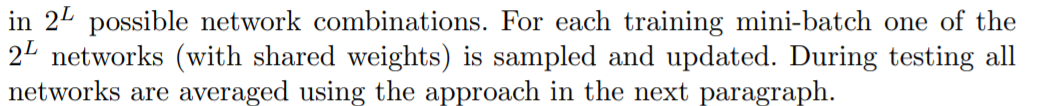
Implicit model ensemble. In addition to the predicted speedups, we also observe significantly lower testing errors in our experiments, in comparison with ResNets of constant depth. One explanation for our performance improvements is that training with stochastic depth can be viewed as training an ensemble of ResNets implicitly. Each of the L layers is either active or inactive, resulting
From the model ensemble perspective, the update rule (5) can be interpreted as combining all possible networks into a single test architecture, in which each layer is weighted by its survival probability.
4 Results
We empirically demonstrate the effectiveness of stochastic depth on a series of benchmark data sets: CIFAR-10, CIFAR-100 [1], SVHN [31], and ImageNet [2].
construction scheme (for constant and stochastic depth) as described by He et al. [8]. In the case of CIFAR-100 we use the same 110-layer ResNet used by He et al. [8] for CIFAR-10, except that the network has a 100-way softmax output. Each model contains three groups of residual blocks that differ in number of filters and feature map size, and each group is a stack of 18 residual blocks. The numbers of filters in the three groups are 16, 32 and 64, respectively. For the transitional residual blocks, i.e. the first residual block in the second and third group, the output dimension is larger than the input dimension. Following He et al. [8], we replace the identity connections in these blocks by an average pooling layer followed by zero paddings to match the dimensions. Our implementations are in Torch 7 [32]. The code to reproduce the results is publicly available on GitHub at https://github.com/yueatsprograms/Stochastic_Depth.
CIFAR-10.
dataset of 32-by-32 color images
10 classes of natural scene objects
The training set and test set contain 50,000 and 10,000 images, respectively We hold out 5,000 images as validation set, and use the remaining 45,000 as training samples.Horizontal flipping and translation by 4 pixels are the two standard data augmentation techniques adopted in our experiments, following the common practice [6, 13, 20, 21, 24, 26, 30].
The baseline ResNet is trained with SGD for 500 epochs, with a mini-batch size 128.
The initial learning rate is 0.1, and is divided by a factor of 10 after epochs 250 and 375.
weight decay of 1e-4, momentum of 0.9, and Nesterov momentum [33] with 0 dampening, as suggested by [34].
For stochastic depth, the network structure and all optimization settings are exactly the same as the baseline. All settings were chosen to match the setup of He et al. [8].
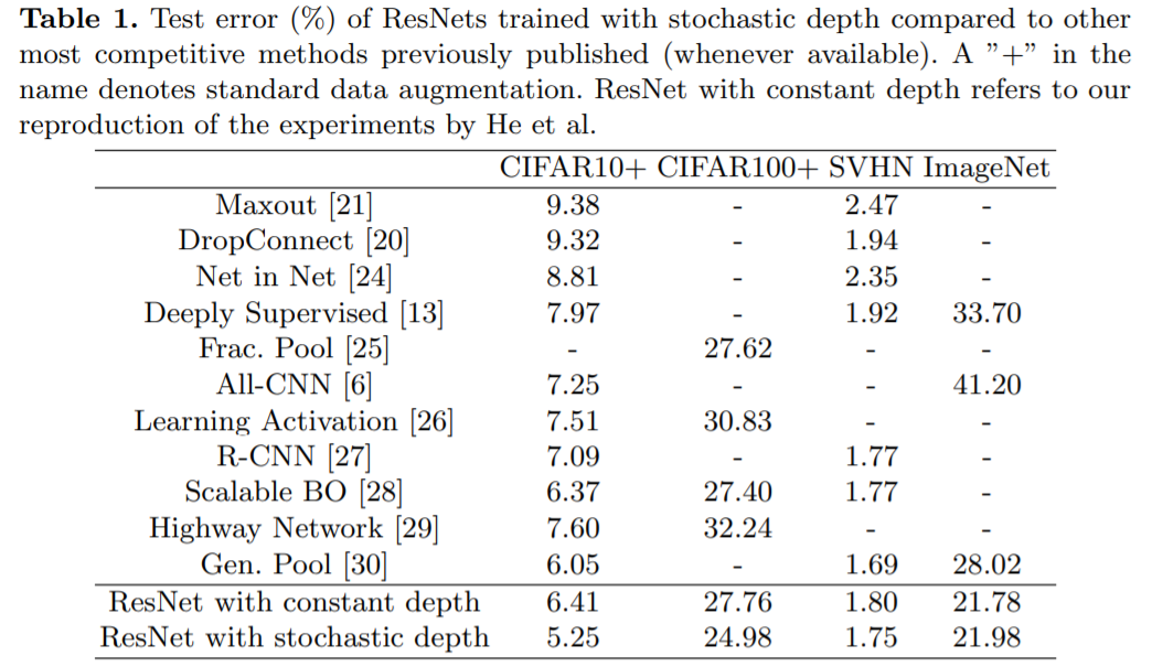
The results are shown in Table 1.
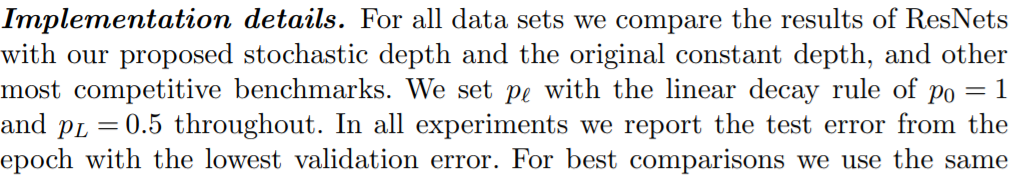
ResNets trained with stochastic depth yield a further relative improvement of 18% and result in 5.25% test error. To our knowledge this is significantly lower than the best existing single model performance (6.05%) [30] on CIFAR-10 prior to our submission, without resorting to massive data augmentation [6, 25].1 Fig. 3 (left) shows the test error as a function of epochs. The point selected by the lowest validation error is circled for both approaches. We observe that ResNets with stochastic depth yield lower test error but also slightly higher fluctuations (presumably due to the random depth during training).
CIFAR-100. Similar to CIFAR-10 color images with the same train-test split, but from 100 classes.
For both the baseline and our method, the experimental settings are exactly the same as those of CIFAR-10. The constant depth ResNet yields a test error of 27.22%, which is already the state-of-the-art in CIFAR-100 with standard data augmentation. Adding stochastic depth drastically reduces the error to 24.98%, and is again the best published single model performance to our knowledge (see Table 1 and Fig. 3 right).
We also experiment with CIFAR-10 and CIFAR-100 without data augmentation. ResNets with constant depth obtain 13.63% and 44.74% on CIFAR-10 and CIFAR-100 respectively. Adding stochastic depth yields consistent improvements of about 15% on both datasets, resulting in test errors of 11.66% and 37.8% respectively.
SVHN. The format of the Street View House Number (SVHN) [31] dataset that
32-by-32 colored images of cropped out house numbers from Google Street View.
The task is to classify the digit at the center.
There are 73,257 digits in the training set, 26,032 in the test set and 531,131 easier samples for additional training. Following the common practice, we use all the training samples but do not perform data augmentation. For each of the ten classes, we randomly select 400 samples from the training set and 200 from the additional set, forming a validation set with 6,000 samples in total. We preprocess the data by subtracting the mean and dividing the standard deviation. Batch size is set to 128, and validation error is calculated every 200 iterations.
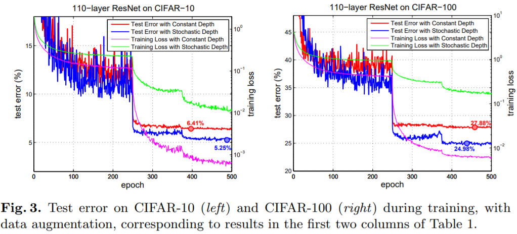
Our baseline network has 152 layers. It is trained for 50 epochs with a beginning learning rate of 0.1, divided by 10 after epochs 30 and 35. The depth and learning rate schedule are selected by optimizing for the validation error of the baseline through many trials. This baseline obtains a competitive result of 1.80%. However, as seen in Fig. 4, it starts to overfit at the beginning of the second phase with learning rate 0.01, and continues to overfit until the end of training. With stochastic depth, the error improves to 1.75%, the second-best published result on SVHN to our knowledge after [30].
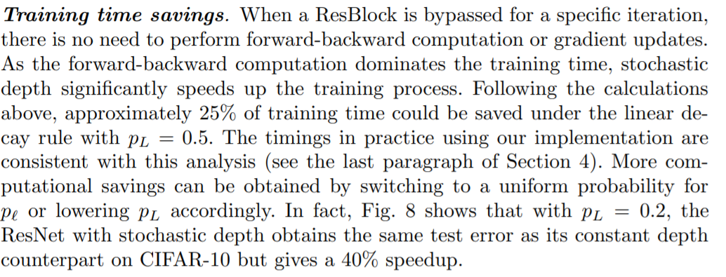
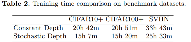
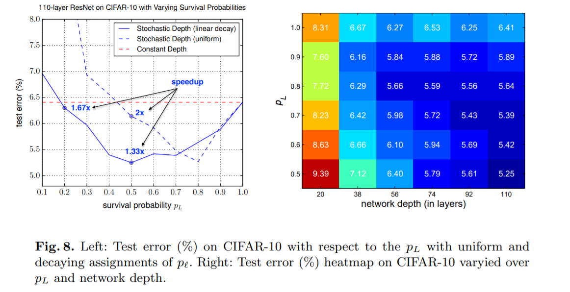
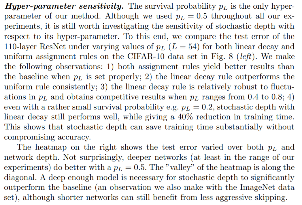
Training time comparison. We compare the training efficiency of the constant depth and stochastic depth ResNets used to produce the previous results. Table 2 shows the training (clock) time under both settings with the linear decay rule pL = 0.5. Stochastic depth consistently gives a 25% speedup, which confirms our analysis in Section 3. See Fig. 8 and the corresponding section on hyper-parameter sensitivity for more empirical analysis.
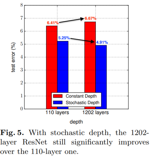
Training with a 1202-layer ResNet. He et al. [8] tried to learn CIFAR10 using an aggressively deep ResNet with 1202 layers. As expected, this extremely deep network overfitted to the training set: it ended up with a test error of 7.93%, worse than their 110- layer network. We repeat their experiment on the same 1202-layer network, with constant and stochastic depth. We train for 300 epochs, and set the learning rate to 0.01 for the first 10 epochs to “warm-up” the network and facilitate initial convergence, then restore it to 0.1, and divide it by 10 at epochs 150 and 225.
The results are summarized in Fig. 4 (right) and Fig. 5. Similar to He et al. [8], the ResNets with constant depth of 1202 layers yields a test error of 6.67%, which is worse than the 110-layer constant depth ResNet. In contrast, if trained with stochastic depth, this extremely deep ResNet performs remarkably well. We want to highlight two trends: 1) Comparing the two 1202-layer nets shows that training with stochastic depth leads to a 27% relative improvement; 2)
ImageNet.
The ILSVRC 2012 classification dataset consists of 1000 classes of images, in total 1.2 million for training, 50,000 for validation, and 100,000 for testing. Following the common practice, we only report the validation errors. We follow He et al. [8] to build a 152-layer ResNet with 50 bottleneck residual blocks. When input and output dimensions do not match, the skip connection uses a learned linear projection for the mismatching dimensions, and an identity transformation for the other dimensions. Our implementation is based on the github repository fb.resnet.torch [34], and the optimization settings are the same as theirs, except that we use a batch size of 128 instead of 256 because we can only spread a batch among 4 GPUs (instead of 8 as they did).
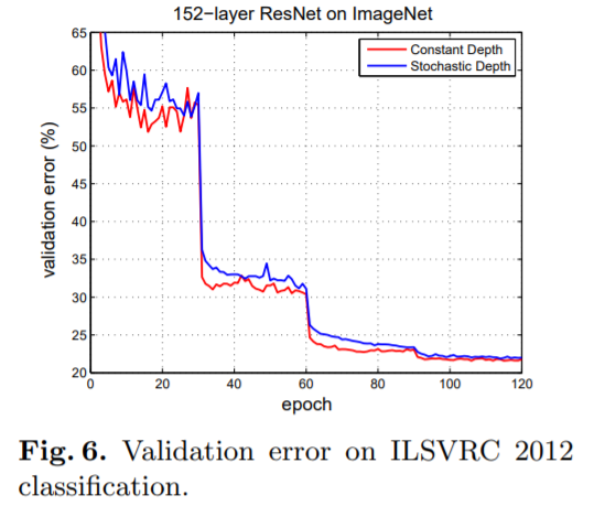
We train the constant depth baseline for 90 epochs (following He et al. and the default setting in the repository) and obtain a final error of 23.06%. With stochastic depth, we obtain an error of 23.38% at epoch 90, which is slightly higher. We observe from Fig.6 that the downward trend of the validation error with stochastic depth is still strong, and from our previous experience, could benefit from further training. Due to the 25% computational saving, we can add 30 epochs (giving 120 in total, after decreasing the learning rate to 1e-4 at epoch 90), and still finish in almost the same total time as 90 epochs of the baseline. This reaches a final error of 21.98%. We have also kept the baseline running for 30 more epochs. This reaches a final error of 21.78%.
Because ImageNet is a very complicated and large dataset, the model complexity required could potentially be much more than that of the 152-layer ResNet [35]. In the words of an anonymous reviewer, the current generation of models for ImageNet are still in a different regime from those of CIFAR. Although there seems to be no immediate benefit from applying stochastic depth on this particular architecture, it is possible that stochastic depth will lead to improvements on ImageNet with larger models, which the community might soon be able to train as GPU capacities increase.
5 Analytic Experiments
we provide more insights into stochastic depth by presenting a series of analytical results. We perform experiments to support the hypothesis that stochastic depth effectively addresses the problem of vanishing gradients in backward propagation. Moreover, we demonstrate the robustness of stochastic depth with respect to its hyper-parameter.
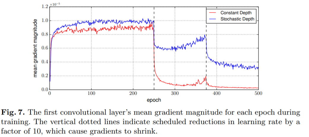
Fig. 7 shows the mean absolute values of the gradients. The two large drops indicated by vertical dotted lines are due to scheduled learning rate division. It can be observed that the magnitude of gradients in the network trained with stochastic depth is always larger, especially after the learning rate drops. This seems to support out claim that stochastic depth indeed significantly reduces the vanishing gradient problem, and enables the network to be trained more effectively. Another indication of the effect is in the left panel of Fig. 3, where one can observe that the test error of the ResNets with constant depth approximately plateaus after the first drop of learning rate, while stochastic depth still improves the performance even after the learning rate drops for the second time. This further supports that stochastic depth combines the benefits of shortened network during training with those of deep models at test time.
6 Conclusion In this paper we introduced deep networks with stochastic depth, a procedure to train very deep neural networks effectively and efficiently. Stochastic depth reduces the network depth during training in expectation while maintaining the full depth at testing time. Training with stochastic depth allows one to increase the depth of a network well beyond 1000 layers, and still obtain a reduction in test error. Because of its simplicity and practicality we hope that training with stochastic depth may become a new tool in the deep learning “toolbox”, and will help researchers scale their models to previously unattainable depths and capabilities.